What is CFD?
Lesson 1.1 of the CFD for Absolute Beginners course — What is CFD?.
Module 1.1 — What is CFD?
The core idea in one sentence: CFD turns the continuous physics of fluid flow — described by partial differential equations — into a finite set of numbers that a computer can crunch.
Why this matters before anything else: Every solver you write in this curriculum is doing one thing: approximating reality with numbers on a grid. If you don't understand why that approximation is necessary, you will misuse every result it gives you.
What this module covers:
- Why analytical solutions to fluid equations are essentially impossible for real geometries
- The mosaic idea — how discretisation makes the impossible tractable
- The six-step CFD pipeline — the mental model for everything that follows
- CFD vs. experiment vs. theory — what each method is actually good for
- What the Navier-Stokes equations say in plain English
- A first look at a real CFD solution
import numpy as np
import matplotlib.pyplot as plt
1. Why Analytical Solutions Are Rare
The textbook illusion
In a fluids textbook you can solve for the velocity profile in a pipe (Hagen-Poiseuille), the drag on a sphere at very low speed (Stokes drag), or the lift on an infinite flat plate (thin-airfoil theory). These are elegant closed-form results. They suggest that with enough cleverness you could always find a formula.
That impression is completely wrong.
All those textbook solutions share two features: trivially simple geometry (infinite plate, infinite pipe, perfect sphere) and strong simplifying assumptions (steady, incompressible, inviscid, laminar, 2D, ...). Remove even one of those assumptions — put a bump on the pipe wall, add a corner, let the flow become turbulent — and the analytical solution vanishes.
Why the Navier-Stokes equations resist analysis
The momentum equation for an incompressible fluid is:
The highlighted term — the nonlinear convective term — is the problem. It means: the velocity field transports itself. The flow carries the very momentum that determines how it flows. This circularity creates a nonlinear PDE where the unknown () appears multiplied by its own derivative. Nonlinear PDEs almost never have exact solutions for non-trivial domains.
This is not a gap in our mathematical knowledge — it is a structural property of the equations. The Clay Mathematics Institute has offered $1,000,000 to anyone who can prove (or disprove) that smooth solutions to 3D N-S always exist. As of 2025, the prize is unclaimed.
The CFD way out
Instead of solving the PDE exactly everywhere, CFD solves it approximately at a finite number of points. The continuous domain is replaced by a discrete grid; continuous derivatives are replaced by algebraic differences between neighbouring grid values; and the PDE becomes a large system of ordinary equations that a computer can solve.
The approximation can be made as accurate as desired by refining the grid. The cost of doing so is more computation — this is the fundamental trade-off in all of CFD.
2. The Mosaic Idea — Discretisation
The analogy
A mosaic reproduces the Mona Lisa using square tiles. Each tile is completely described by one colour — a single number. The combination of thousands of trivially simple tiles captures the full complexity of the original painting.
CFD does the same thing with physics.
Continuous domain                 Discretised domain
────────────────────              ────────────────────
u(x,y,t) — a function that        u[i,j,n] — a 3D array of
varies continuously at            numbers, one per grid
every point in space and time     point per time step

∂u/∂x — a derivative             (u[i+1,j] - u[i-1,j])/(2Δx)
defined at every point            — a difference between
                                  neighbouring array values

∂²u/∂x² — smooth curvature       (u[i+1,j]-2u[i,j]+u[i-1,j])/Δx²
                                  — one algebraic expression
What is lost — and what is gained
| Property | Continuous PDE | Discrete CFD |
|---|---|---|
| Solution space | Infinitely many values | Finite array |
| Exactness | Exact (if solvable) | Approximate — error |
| Geometry | Any shape, in principle | Constrained by grid |
| Solvable for real problems? | Almost never | Yes, always |
| Can be refined? | N/A | Yes — halve , error decreases |
The error in CFD goes to zero as the grid is refined. A coarse grid gives a rough answer; a fine grid gives a precise one. This is called convergence and it is how you know your CFD result is trustworthy.
3. The Six-Step CFD Pipeline
Every CFD simulation — from a student exercise to a full aircraft simulation — follows this sequence. Memorise it now, because every notebook in this curriculum maps onto these six steps.
STEP 1 — Geometry
  Define the shape of the fluid domain.
  (Unit square for cavity, airfoil profile for aero, pipe cross-section for heat transfer)

STEP 2 — Mesh generation
  Divide the domain into cells.
  Mesh quality controls both accuracy and solver stability.
  (Module 3.3 covers this in depth)

STEP 3 — Physics setup
  Choose which equations to solve (N-S, energy, turbulence transport)
  and set fluid properties (ρ, μ, k, cp).

STEP 4 — Boundary and initial conditions
  Tell the solver what happens at every boundary (inlet velocity, wall temperature, etc.)
  and what the flow looks like at t = 0.
  WRONG BCs → WRONG PHYSICS, even if the solver is perfect.

STEP 5 — Solve
  Run the iterative solver until residuals converge.
  Residual = how much the current solution violates the governing equations.
  Converged = residuals < 10⁻⁶ (typical criterion).

STEP 6 — Post-process
  Extract numbers (drag, heat flux, pressure drop) and visualise fields
  (velocity vectors, pressure contours, temperature maps).
  ALWAYS verify against an analytical solution or experiment before trusting results.
Steps 1–4 are pre-processing (typically 60–80% of the engineer's time in industrial CFD). Step 5 is the solver (automated, often runs overnight). Step 6 is post-processing (interpreting what the numbers mean physically).
This curriculum covers all six steps.
4. The Navier-Stokes Equations in Plain English
The governing equations of incompressible flow are two statements:
Statement 1 — Continuity (mass conservation)
Plain English: For every fluid parcel, what flows in must flow out. The velocity field has zero divergence — fluid is not created or destroyed anywhere.
In 2D: — if the flow speeds up in , it must slow down in to compensate.
Statement 2 — Momentum (Newton's second law)
Plain English: The left side is per unit volume — the rate of change of a fluid parcel's momentum as it moves. The right side is the total force per unit volume: pressure gradient (fluid pushed from high to low pressure) plus viscous friction (fast layers drag slow layers).
Why the convective term is special: means "the current velocity field advects the velocity field itself." This self-referential, nonlinear term is the source of turbulence, instability, and every interesting flow phenomenon. Remove it and you get Stokes flow — trivially solvable but physically uninteresting.
The Reynolds number tells you which term dominates
Non-dimensionalise with velocity scale and length scale . The ratio of convection to viscosity is:
- : viscosity dominates, flow is smooth and creeping (swimming bacteria, MEMS devices)
- –: both terms matter, laminar with structure (your cavity solver)
- : inertia dominates, flow becomes turbulent
- (aircraft): inertia crushes viscosity except in a thin layer near the wall
# ── A first look at a CFD solution ──────────────────────────────────────────
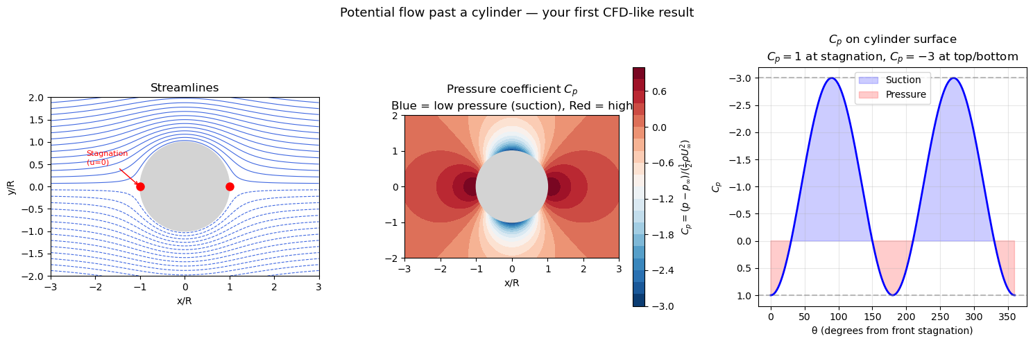
# Potential flow past a cylinder: an analytical solution for inviscid flow.
# This is NOT a numerical CFD solve — it shows what CFD results look like
# and introduces the vocabulary (streamlines, stagnation, pressure coefficient).
# ── Grid ────────────────────────────────────────────────────────────────────
x = np.linspace(-3, 3, 400)
y = np.linspace(-2, 2, 300)
X, Y = np.meshgrid(x, y)
R = 1.0 # cylinder radius
U_inf = 1.0 # freestream speed
Z = X + 1j * Y
# ── Potential flow complex potential: w = U∞(z + R²/z) ──────────────────────
# Inside cylinder: set to nan so it plots as a solid body
mask = (X**2 + Y**2) < R**2
Z_safe = np.where(mask, np.nan + 0j, Z)
W = U_inf * (Z_safe + R**2 / Z_safe)
psi = W.imag # streamfunction — contours of this are streamlines
phi = W.real # velocity potential
# ── Velocity components: u = ∂φ/∂x, v = ∂φ/∂y ─────────────────────────────
dw_dz = U_inf * (1 - R**2 / Z_safe**2) # complex velocity
u_field = dw_dz.real
v_field = -dw_dz.imag
speed = np.sqrt(u_field**2 + v_field**2)
# ── Pressure coefficient: Cp = 1 - (V/U∞)² ─────────────────────────────────
Cp = 1 - (speed / U_inf)**2
Cp[mask] = np.nan
# ── Plots ────────────────────────────────────────────────────────────────────
fig, axes = plt.subplots(1, 3, figsize=(15, 5))
# Left — streamlines
levels = np.linspace(-2.5, 2.5, 40)
axes[0].contour(X, Y, psi, levels=levels, colors='royalblue', linewidths=0.8)
axes[0].add_patch(plt.Circle((0,0), R, color='lightgray', zorder=5))
axes[0].set_aspect('equal'); axes[0].set_xlim(-3,3); axes[0].set_ylim(-2,2)
axes[0].set_title('Streamlines')
axes[0].set_xlabel('x/R'); axes[0].set_ylabel('y/R')
# Mark stagnation points
axes[0].plot([-1,1],[0,0],'ro', markersize=8, zorder=6)
axes[0].annotate('Stagnation\n(u=0)', xy=(-1,0), xytext=(-2.2, 0.5), fontsize=8,
arrowprops=dict(arrowstyle='->', color='red'), color='red')
# Middle — pressure coefficient
cf = axes[1].contourf(X, Y, Cp, levels=20, cmap='RdBu_r', vmin=-3, vmax=1)
plt.colorbar(cf, ax=axes[1], label='$C_p = (p-p_\\infty)/(\\frac{1}{2}\\rho U_\\infty^2)$')
axes[1].add_patch(plt.Circle((0,0), R, color='lightgray', zorder=5))
axes[1].set_aspect('equal'); axes[1].set_xlim(-3,3); axes[1].set_ylim(-2,2)
axes[1].set_title('Pressure coefficient $C_p$\nBlue = low pressure (suction), Red = high')
axes[1].set_xlabel('x/R')
# Right — Cp on cylinder surface
theta = np.linspace(0, 2*np.pi, 360)
Cp_surface = 1 - 4*np.sin(theta)**2 # exact: Cp = 1 - 4sin²θ
axes[2].plot(np.degrees(theta), Cp_surface, 'b-', linewidth=2)
axes[2].axhline(-3, color='gray', linestyle='--', alpha=0.5)
axes[2].axhline(1, color='gray', linestyle='--', alpha=0.5)
axes[2].fill_between(np.degrees(theta), Cp_surface, 0,
where=Cp_surface<0, alpha=0.2, color='blue', label='Suction')
axes[2].fill_between(np.degrees(theta), Cp_surface, 0,
where=Cp_surface>0, alpha=0.2, color='red', label='Pressure')
axes[2].set_xlabel('θ (degrees from front stagnation)')
axes[2].set_ylabel('$C_p$')
axes[2].set_title('$C_p$ on cylinder surface\n$C_p=1$ at stagnation, $C_p=-3$ at top/bottom')
axes[2].legend(); axes[2].grid(True, alpha=0.3)
axes[2].invert_yaxis() # convention: Cp axis runs downward
plt.suptitle('Potential flow past a cylinder — your first CFD-like result', fontsize=13)
plt.tight_layout()
plt.show()
print('Key observations:')
print(' 1. Flow is perfectly symmetric — no wake. This is inviscid (ν=0).')
print(' With viscosity, a wake forms (Module 2.7 shows this).')
print(' 2. Cp=1 at front stagnation — all kinetic energy converts to pressure.')
print(' By Bernoulli: p + ½ρu² = const → u=0 gives max p.')
print(' 3. Cp=-3 at top and bottom — flow accelerates around the cylinder,')
print(' lowering pressure. This is the mechanism of LIFT.')
print(' 4. Symmetric Cp → net force = 0 (d\'Alembert paradox).')
print(' Real viscous flow breaks the symmetry → drag exists.')
/var/folders/j6/slfvk4c54yj6lt99pq5rjh8m0000gn/T/ipykernel_6868/1128790559.py:19: RuntimeWarning: invalid value encountered in divide
  W   = U_inf * (Z_safe + R**2 / Z_safe)
/var/folders/j6/slfvk4c54yj6lt99pq5rjh8m0000gn/T/ipykernel_6868/1128790559.py:24: RuntimeWarning: invalid value encountered in divide
  dw_dz = U_inf * (1 - R**2 / Z_safe**2)   # complex velocity
Key observations:
  1. Flow is perfectly symmetric — no wake. This is inviscid (ν=0).
     With viscosity, a wake forms (Module 2.7 shows this).
  2. Cp=1 at front stagnation — all kinetic energy converts to pressure.
     By Bernoulli: p + ½ρu² = const → u=0 gives max p.
  3. Cp=-3 at top and bottom — flow accelerates around the cylinder,
     lowering pressure. This is the mechanism of LIFT.
  4. Symmetric Cp → net force = 0 (d'Alembert paradox).
     Real viscous flow breaks the symmetry → drag exists.
5. CFD vs. Experiment vs. Theory
Each approach answers different questions and has different failure modes. A good engineer uses all three.
| Method | Best for | Key limitations | Typical cost |
|---|---|---|---|
| Theory | Fundamental understanding; scaling laws; design intuition | Only works for simplified geometries | Zero (pencil + paper) |
| Experiment | Ground truth; complex flows; discovering unexpected physics | Expensive; hard to change parameters; limited measurement access | High (wind tunnels: €1k–€100k/day) |
| CFD | Complex geometries; parametric studies; flow visualisation inside solid walls | Only as good as the model; requires validation against experiment | Medium (compute: €1–€1000/simulation) |
Where CFD fails — the most important thing to know before you trust a result
CFD gives you a result for every input you give it. Wrong BCs, wrong turbulence model, under-resolved mesh — it still converges and gives you beautiful contour plots. The answer will be wrong, but it won't look wrong.
The only protection is validation: always compare your CFD result against an analytical solution (when one exists) or experimental data. Until you have done this, your result is a hypothesis, not a prediction.
Every module in this curriculum includes a validation step. This is not optional.
6. Where Each Module Fits in the Pipeline
Module 1.1 (this)  — What CFD is and why it works
Module 1.2         — Python tools: NumPy arrays, vectorisation, Matplotlib
Modules 1.3–1.4    — Conservation laws: the physics behind every equation
Module 1.5         — Finite differences: converting PDEs to algebra
Modules 1.6–1.8    — 1D PDEs: advection, diffusion, Burgers (nonlinear)
Module 2.1         — 2D extension: same equations, new indexing complexity
Modules 2.2–2.6    — Incompressible N-S solver from scratch (FVM + SIMPLE)
Modules 2.7–2.8    — External flow: cylinder, boundary conditions
Modules 3.1–3.2    — Turbulence: RANS equations and models
Modules 3.3–3.8    — Advanced: meshing, higher-order schemes, compressible flow
Module 4           — Complete engineering projects
Summary
| Concept | Key point |
|---|---|
| Why CFD | N-S equations have no general analytical solution for real geometries |
| How CFD | Discretise the domain into cells; replace derivatives with algebraic differences |
| Accuracy | Error — halve grid spacing, error drops by |
| Pipeline | 6 steps: geometry → mesh → physics → BCs → solve → post-process |
| Governing eq. | Continuity () + Momentum (Newton's 2nd law per unit volume) |
| Reynolds number | — ratio of inertia to viscosity; controls the flow regime |
| Critical rule | Always validate — a CFD result without validation is a hypothesis |
Next: Module 1.2 — Python for CFD: NumPy arrays, vectorised operations, and the slice patterns you will use in every solver.