1D Burgers Equation
Lesson 1.8 of the CFD for Absolute Beginners course — 1D Burgers Equation.
Module 1.8 — 1D Burgers' Equation
The equation that connects everything:
Burgers' equation is the 1D prototype of the Navier-Stokes equations. It contains:
- — the nonlinear convective term (same form as in N-S)
- — viscous diffusion (same form as in N-S)
Everything you learn in this module carries over directly to the full N-S equations in Module 2.
Roadmap:
- Physical intuition — the traffic jam mechanism of shock formation
- Conservative vs. non-conservative form — why it matters for shocks
- Characteristics — how information propagates in nonlinear equations
- Inviscid case (): shock formation and the Rankine-Hugoniot condition
- Viscous case (): the shock structure and the Reynolds number analogy
- Implementation: explicit scheme with shock capturing
- Connection to Navier-Stokes
import numpy as np
import matplotlib.pyplot as plt
1. The Traffic Jam Analogy
Why nonlinearity causes shocks
In linear advection (Module 1.6), every part of the initial profile moves at the same speed . The shape is preserved.
In Burgers' equation, each part of the profile moves at its own speed — the local value of . A region where moves twice as fast as a region where .
Imagine cars on a highway:
Fast cars  →→→→→→→→→→→→  Slow cars ahead
                         ↓
Fast cars catch up → PILE-UP = SHOCK
In fluid terms: the high-velocity region of the initial wave catches up to the low-velocity region ahead of it. The wave steepens until it becomes a vertical front — a shock.
Shock formation time
For the inviscid equation, the characteristics are lines . Two characteristics starting at and meet at time:
If the initial profile has a negative slope anywhere (), a shock forms in finite time. The shock formation time is determined by the steepest downslope in the initial condition.
For : at , so .
2. Conservative vs. Non-Conservative Form
Two ways to write the same equation
Non-conservative (advective) form:
Conservative (divergence) form:
For smooth solutions, these are equivalent (product rule: ).
Why it matters at shocks
At a shock, is discontinuous. The derivative does not exist in the classical sense — you cannot compute point-by-point.
The conservative form avoids this: can be interpreted in the weak (integral) sense even when is discontinuous. The correct shock speed (Rankine-Hugoniot condition) is obtained only from the conservative form:
where and are the values on the left and right of the shock.
Rule: always discretise the convective term in conservation form. Non-conservative schemes give the wrong shock speed.
This rule applies directly to the Navier-Stokes equations: the momentum equation must be in conservative form (, not ) for correct shock-capturing in compressible flow.
3. The Viscous Burgers Equation and the Reynolds Number Analogy
What viscosity does to a shock
Adding viscosity () regularises the shock: instead of a discontinuity, there is a thin smooth transition layer. The thickness of this layer scales as:
where is the velocity jump across the shock.
The ratio of the shock amplitude to the viscous thickness defines a shock Reynolds number:
At the shock, inertia and viscosity are exactly balanced — this is the same balance that defines the thickness of a laminar boundary layer. The analogy with the N-S Reynolds number is not a coincidence — Burgers' equation is the N-S equations reduced to 1D.
The exact solution for any
The Cole-Hopf transformation converts Burgers' to the linear heat equation. The exact solution for sinusoidal IC is:
At small : the solution develops a sharp internal layer (shock). At large : viscosity smooths everything quickly and the solution decays like a heat equation.
# ── Burgers' equation solver ─────────────────────────────────────────────────
# Conservative form: ∂u/∂t + ∂(u²/2)/∂x = ν∂²u/∂x²
# Lax-Friedrichs for convective flux (conservative, handles shocks)
# Explicit central for diffusion
def burgers_solve(u0, nu, dx, T, cfl_convection=0.4, cfl_diffusion=0.4):
"""
Solve viscous Burgers' equation using conservative Lax-Friedrichs flux.
Time step chosen to satisfy both CFL conditions.
"""
u = u0.copy()
N = len(u)
t = 0.0
while t < T:
umax = np.max(np.abs(u)) + 1e-10
# CFL for convection: dt < dx / max|u|
dt_conv = cfl_convection * dx / umax
# Stability for diffusion: dt < dx² / (2ν)
dt_diff = cfl_diffusion * dx**2 / (2*nu + 1e-12)
dt = min(dt_conv, dt_diff, T - t)
un = u.copy()
# ── Conservative Lax-Friedrichs flux at faces ───────────────────────
# F(u) = u²/2
F = 0.5 * un**2
# Lax-Friedrichs: F_{i+1/2} = (F_i + F_{i+1})/2 - (dx/2dt)*(u_{i+1}-u_i)
# The dissipation term makes the scheme conservative AND stable
speed = umax # max wave speed for diffusion
F_right = 0.5*(F[1:] + F[:-1]) - 0.5*(dx/dt)*speed*(un[1:] - un[:-1])
# ── Update interior from flux balance ───────────────────────────────
u[1:-1] = un[1:-1] - dt/dx*(F_right[1:] - F_right[:-1])
# ── Diffusion (explicit, central) ────────────────────────────────────
u[1:-1] += dt * nu * (un[2:] - 2*un[1:-1] + un[:-2]) / dx**2
# ── BCs: periodic ────────────────────────────────────────────────────
u[0] = u[-2]; u[-1] = u[1]
t += dt
return u
# ── Setup: sine wave IC on [0, 2π] ───────────────────────────────────────────
N = 300
L = 2 * np.pi
dx = L / N
x = np.linspace(0, L, N, endpoint=False)
u0 = np.sin(x)
# Shock formation time for u0=sin(x): t_s = 1
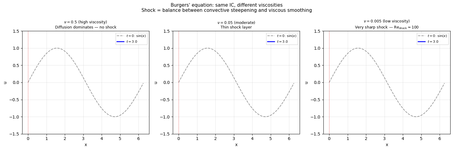
fig, axes = plt.subplots(1, 3, figsize=(15, 5))
viscosities = [0.5, 0.05, 0.005]
titles = [
'$\\nu = 0.5$ (high viscosity)\nDiffusion dominates — no shock',
'$\\nu = 0.05$ (moderate)\nThin shock layer',
'$\\nu = 0.005$ (low viscosity)\nVery sharp shock — Re$_{\\mathrm{shock}} \\approx 100$'
]
for ax, nu, title in zip(axes, viscosities, titles):
T_final = 3.0
u_final = burgers_solve(u0, nu, dx, T_final)
ax.plot(x, u0, 'k--', lw=1.5, alpha=0.4, label='$t=0$: $\\sin(x)$')
ax.plot(x, u_final, 'b-', lw=2, label=f'$t={T_final}$')
ax.set_title(title, fontsize=9)
ax.set_xlabel('x'); ax.set_ylabel('u')
ax.legend(fontsize=8); ax.grid(True, alpha=0.3)
ax.set_ylim(-1.5, 1.5)
# Mark approximate shock location and width
grad = np.gradient(u_final, dx)
i_shock = np.argmin(grad)
ax.axvline(x[i_shock], color='r', lw=1, linestyle=':', alpha=0.7)
plt.suptitle("Burgers' equation: same IC, different viscosities\n"
'Shock = balance between convective steepening and viscous smoothing', fontsize=11)
plt.tight_layout()
plt.show()
print('\nViscosity is the Reynolds number dial:')
for nu in viscosities:
Re_shock = 1.0 / (nu + 1e-10) # ΔU ~ 1, δ ~ ν
print(f' ν={nu:6.3f} → Re_shock ~ {Re_shock:.0f} → ',
'diffusion dominates' if nu >= 0.1 else 'sharp shock')
/var/folders/j6/slfvk4c54yj6lt99pq5rjh8m0000gn/T/ipykernel_6943/1052683741.py:31: RuntimeWarning: overflow encountered in multiply
  F_right = 0.5*(F[1:] + F[:-1]) - 0.5*(dx/dt)*speed*(un[1:] - un[:-1])
/var/folders/j6/slfvk4c54yj6lt99pq5rjh8m0000gn/T/ipykernel_6943/1052683741.py:34: RuntimeWarning: invalid value encountered in subtract
  u[1:-1] = un[1:-1] - dt/dx*(F_right[1:] - F_right[:-1])
Viscosity is the Reynolds number dial:
  ν= 0.500  →  Re_shock ~ 2  →   diffusion dominates
  ν= 0.050  →  Re_shock ~ 20  →   sharp shock
  ν= 0.005  →  Re_shock ~ 200  →   sharp shock
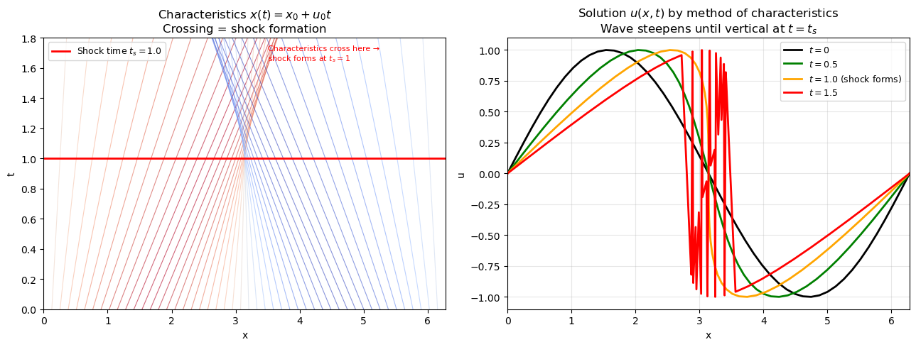
# ── Characteristics: visualise shock formation from first principles ─────────
# x(t) = x₀ + u₀(x₀)·t — characteristic lines cross at t = t_shock

x0_vals = np.linspace(0, 2*np.pi, 50)
u0_vals = np.sin(x0_vals)
t_shock = 1.0   # for u0=sin(x): -1/min(u0') = -1/(-1) = 1

t_range = np.linspace(0, 1.8, 100)

fig, axes = plt.subplots(1, 2, figsize=(13, 5))

# Left: characteristic lines in (x, t) space
for x0, u0 in zip(x0_vals, u0_vals):
    x_char = x0 + u0 * t_range
    color = plt.cm.coolwarm(0.5 + 0.5*u0)  # colour by initial velocity
    axes[0].plot(x_char, t_range, '-', color=color, lw=0.8, alpha=0.6)

axes[0].axhline(t_shock, color='red', lw=2, label=f'Shock time $t_s = {t_shock}$')
axes[0].set_xlabel('x'); axes[0].set_ylabel('t')
axes[0].set_title('Characteristics $x(t) = x_0 + u_0 t$\n'
                   'Crossing = shock formation')
axes[0].legend(fontsize=9)
axes[0].set_xlim(0, 2*np.pi); axes[0].set_ylim(0, 1.8)
axes[0].text(3.5, 1.65, 'Characteristics cross here →\nshock forms at $t_s=1$',
             fontsize=8, color='red')

# Right: solution profiles at different times
times = [0, 0.5, 1.0, 1.5]
colors_t = ['black', 'green', 'orange', 'red']
for t_plot, color in zip(times, colors_t):
    # Method of characteristics (valid for t < t_shock)
    x_char = x0_vals + u0_vals * t_plot
    idx    = np.argsort(x_char)
    label  = f'$t={t_plot}$' + (' (shock forms)' if t_plot == 1.0 else '')
    axes[1].plot(x_char[idx], u0_vals[idx], '-', color=color, lw=2, label=label)

axes[1].set_xlabel('x'); axes[1].set_ylabel('u')
axes[1].set_title('Solution $u(x,t)$ by method of characteristics\n'
                   'Wave steepens until vertical at $t=t_s$')
axes[1].legend(fontsize=9); axes[1].grid(True, alpha=0.3)
axes[1].set_xlim(0, 2*np.pi)

plt.tight_layout()
plt.show()

print('After t = t_s = 1.0:')
print('  Inviscid: solution is multi-valued (physically inadmissible)')
print('  Viscous:  thin shock layer resolves the crossing — unique single-valued solution')
print('  Numerical: upwind scheme smears the shock over ~5-10 cells')
After t = t_s = 1.0:
  Inviscid: solution is multi-valued (physically inadmissible)
  Viscous:  thin shock layer resolves the crossing — unique single-valued solution
  Numerical: upwind scheme smears the shock over ~5-10 cells
4. Connection to Navier-Stokes — Why You Studied Burgers' Equation
| Burgers' property | Navier-Stokes equivalent |
|---|---|
| (nonlinear advection) | (convective inertia) |
| (viscous diffusion) | (viscous stress) |
| Reynolds number | Flow Reynolds number |
| Shock = thin internal layer | Boundary layer = thin wall-attached layer |
| Conservative form required | Conservative N-S form required |
| CFL for convection + for diffusion | Same two constraints in 2D N-S |
Every numerical difficulty you encountered in Burgers' — stability, shock smearing, time-step restrictions — appears again in the Navier-Stokes solver. The solutions are the same: upwind for convection, implicit for diffusion, conservative discretisation.
Summary
| Concept | Key point |
|---|---|
| Nonlinearity | : each part of the wave moves at its own speed |
| Shock formation | Occurs in finite time for smooth IC |
| Conservative form | Required for correct shock speed (Rankine-Hugoniot) |
| Viscosity | Regularises shock into a layer of thickness |
| Time step | Must satisfy both (CFL) AND |
| Connection to N-S | Burgers is the 1D N-S; all its difficulties carry over to 2D |
End of Module 1. You have built every scalar PDE solver you need for what comes next.
Next: Module 2.1 — 2D Scalar Transport: extending to two spatial dimensions, structured grids, and the operator-splitting approach.
Exercise
Predict first, then verify.
-
For the initial condition on (a negative slope everywhere): predict from the formula . Run the inviscid solver and confirm the shock appears at that time.
-
The Rankine-Hugoniot condition for Burgers' equation says the shock speed is where and are the values on either side. For the sine-wave IC at : does the shock in your simulation move at the predicted speed?
-
Numerical diffusion effect: Run the same case with (inviscid) using three different grid resolutions (). Does the shock become sharper with finer grid? Measure the shock thickness (width of the transition layer) as a function of . What does this tell you about the numerical diffusion coefficient of the Lax-Friedrichs scheme?