Module 1.5 — Finite Difference Method

The core skill in this module: Turning a derivative on paper into an algebraic expression on a grid. Once you can do this systematically for any derivative, you can discretise any PDE.

Why the FDM before the FVM? FDM is conceptually simpler: derivatives are approximated at grid points. FVM (Module 2.2) is what industrial CFD actually uses. But FDM is the right starting point because you can derive every formula from first principles in five lines, and it gives you physical intuition that FVM obscures.

Roadmap:

Taylor series — the single source of all finite-difference formulas
The three fundamental first-derivative stencils — when to use each
The second derivative — derived from scratch, confirmed experimentally
Truncation error and order of accuracy — what they actually mean
2D stencils and the Laplacian
Convergence study — proving your formula is correct
Ghost cells — handling boundary conditions without special-casing

import numpy as np
import matplotlib.pyplot as plt

1. Taylor Series — The One Source of All FD Formulas

The recipe

Every finite-difference formula comes from the Taylor expansion of a function around a point $x_i$ :

$u(x_i + \Delta x) = u_i + \Delta x\,u'_i + \frac{\Delta x^2}{2}u''_i + \frac{\Delta x^3}{6}u'''_i + \cdots$

Written for the right and left neighbours:

$u_{i+1} = u_i + \Delta x\,u'_i + \frac{\Delta x^2}{2}u''_i + \frac{\Delta x^3}{6}u'''_i + O(\Delta x^4) \quad \text{...(A)}$

$u_{i-1} = u_i - \Delta x\,u'_i + \frac{\Delta x^2}{2}u''_i - \frac{\Delta x^3}{6}u'''_i + O(\Delta x^4) \quad \text{...(B)}$

Three derivative formulas from two expansions

Forward difference — solve (A) for $u'_i$ , drop $O(\Delta x)$ terms: $u'_i = \frac{u_{i+1} - u_i}{\Delta x} - \underbrace{\frac{\Delta x}{2}u''_i + \cdots}_{\text{truncation error}} \implies \boxed{u'_i \approx \frac{u_{i+1} - u_i}{\Delta x}} + O(\Delta x)$

Backward difference — solve (B) for $u'_i$ : $\boxed{u'_i \approx \frac{u_i - u_{i-1}}{\Delta x}} + O(\Delta x)$

Central difference — subtract (B) from (A). The even powers of $\Delta x$ cancel: $(A) - (B): \quad u_{i+1} - u_{i-1} = 2\Delta x\,u'_i + \frac{\Delta x^3}{3}u'''_i + \cdots$ $\boxed{u'_i \approx \frac{u_{i+1} - u_{i-1}}{2\Delta x}} + O(\Delta x^2)$

Central is twice as accurate as forward/backward because the subtraction cancels the $O(\Delta x)$ term. This is always the case: symmetric stencils eliminate even-order error terms.

Second derivative — add (A) and (B). The odd powers cancel: $(A) + (B): \quad u_{i+1} + u_{i-1} = 2u_i + \Delta x^2 u''_i + O(\Delta x^4)$ $\boxed{u''_i \approx \frac{u_{i+1} - 2u_i + u_{i-1}}{\Delta x^2}} + O(\Delta x^2)$

2. When to Use Each Stencil

The choice is not arbitrary — it depends on the physical process being discretised:

Stencil	Formula	Order	Best for	Risk
Forward	$(u_{i+1}-u_i)/\Delta x$	$O(\Delta x)$	Boundary, source terms	One-sided: biases solution
Backward	$(u_i-u_{i-1})/\Delta x$	$O(\Delta x)$	Upwind advection ( $c>0$ )	Numerically diffusive
Central 1st	$(u_{i+1}-u_{i-1})/(2\Delta x)$	$O(\Delta x^2)$	Diffusion terms, pressure	Unstable for pure advection
Central 2nd	$(u_{i+1}-2u_i+u_{i-1})/\Delta x^2$	$O(\Delta x^2)$	All diffusion	None — always use this

The upwind rule for convection

For the advective term $c \cdot \partial u/\partial x$ , always use information from the direction the flow is coming from:

If $c > 0$ (flow goes right): information comes from the left → use backward difference
If $c < 0$ (flow goes left): information comes from the right → use forward difference

# Upwind advection — stable, first-order
if c > 0:
    dudx = (u[1:] - u[:-1]) / dx    # backward
else:
    dudx = (u[1:] - u[:-1]) / dx    # forward (same formula, different interpretation)

# Vectorised with sign detection:
adv = np.where(c > 0,
    c * (u[1:-1] - u[:-2]) / dx,    # backward (c>0)
    c * (u[2:]   - u[1:-1]) / dx)   # forward  (c<0)

Using central differences for advection is unconditionally unstable (Godunov's theorem). Never do it.

# ── Order of accuracy: prove it by measuring the convergence rate ────────────
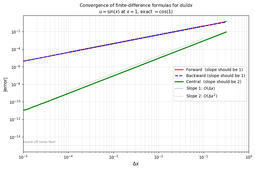
# For u = sin(x), du/dx = cos(x) at x₀ = 1.0
# Theory: forward/backward error ~ dx,  central error ~ dx²

x0    = 1.0
exact = np.cos(x0)

dx_values = np.logspace(-5, -0.5, 60)

err_fwd = []
err_bwd = []
err_cen = []

for dx in dx_values:
    u_plus  = np.sin(x0 + dx)
    u_0     = np.sin(x0)
    u_minus = np.sin(x0 - dx)

    fwd = (u_plus  - u_0    ) / dx
    bwd = (u_0     - u_minus) / dx
    cen = (u_plus  - u_minus) / (2*dx)

    err_fwd.append(abs(fwd - exact))
    err_bwd.append(abs(bwd - exact))
    err_cen.append(abs(cen - exact))

# ── Plot on log-log axes — order appears as slope ────────────────────────────
fig, ax = plt.subplots(figsize=(9, 6))

ax.loglog(dx_values, err_fwd, 'r-',  lw=2,   label='Forward  (slope should be 1)')
ax.loglog(dx_values, err_bwd, 'b--', lw=2,   label='Backward (slope should be 1)')
ax.loglog(dx_values, err_cen, 'g-',  lw=2.5, label='Central  (slope should be 2)')

# Reference lines with known slopes
ref_x = np.array([1e-4, 1e-1])
ax.loglog(ref_x, 0.5  * ref_x**1, 'k--', lw=1, alpha=0.6, label='Slope 1: $O(\\Delta x)$')
ax.loglog(ref_x, 0.17 * ref_x**2, 'k:',  lw=1, alpha=0.6, label='Slope 2: $O(\\Delta x^2)$')

# Round-off noise floor
ax.axhline(1e-15, color='gray', lw=0.5, linestyle=':')
ax.text(1e-5, 2e-15, 'round-off noise floor', fontsize=8, color='gray')

ax.set_xlabel('$\\Delta x$', fontsize=12)
ax.set_ylabel('|error|', fontsize=12)
ax.set_title('Convergence of finite-difference formulas for $du/dx$\n'
             '$u = \\sin(x)$ at $x=1$, exact $= \\cos(1)$', fontsize=11)
ax.legend(fontsize=10); ax.grid(True, which='both', alpha=0.3)
ax.set_xlim([1e-5, 1])
plt.tight_layout()
plt.show()

# ── Measure the actual slopes ────────────────────────────────────────────────
# Estimate slope from middle of the clean convergence region
i1, i2 = 10, 40
slope_fwd = np.log(err_fwd[i2]/err_fwd[i1]) / np.log(dx_values[i2]/dx_values[i1])
slope_cen = np.log(err_cen[i2]/err_cen[i1]) / np.log(dx_values[i2]/dx_values[i1])

print(f'Measured convergence slopes:')
print(f'  Forward  difference: slope = {slope_fwd:.2f}  (theory: 1.00)')
print(f'  Central  difference: slope = {slope_cen:.2f}  (theory: 2.00)')
print()
print('When Δx < ~1e-8: round-off dominates — making Δx smaller makes things WORSE.')
print('Optimal Δx for floating-point: ~√(machine_eps) ≈ 1e-8 for single, 1e-4 for double.')

Measured convergence slopes:
  Forward  difference: slope = 1.00  (theory: 1.00)
  Central  difference: slope = 2.00  (theory: 2.00)

When Δx < ~1e-8: round-off dominates — making Δx smaller makes things WORSE.
Optimal Δx for floating-point: ~√(machine_eps) ≈ 1e-8 for single, 1e-4 for double.

3. Truncation Error vs. Round-Off Error

Two sources of error in FD

Truncation error — comes from dropping higher-order Taylor terms:

$\text{Truncation error} = \frac{\Delta x^p}{c} \cdot u^{(p+1)}$

This decreases as $\Delta x \to 0$ . Making the grid finer always reduces it.

Round-off error — the finite precision of floating-point arithmetic. For IEEE double precision, each subtraction introduces error $\sim 10^{-16} |u|$ .

For the central difference $u' \approx (u_{i+1}-u_{i-1})/(2\Delta x)$ :

Numerator error: $\sim 2\epsilon_m u$ where $\epsilon_m \approx 2.2\times10^{-16}$
Round-off contribution: $\sim \epsilon_m u / \Delta x$

The sweet spot: round-off decreases as $\Delta x$ increases; truncation decreases as $\Delta x$ decreases. Minimum total error is at:

$\Delta x^* \approx \left(\frac{p\,\epsilon_m}{u^{(p+1)}}\right)^{1/(p+1)}$

For central differences ( $p=2$ ): $\Delta x^* \approx \epsilon_m^{1/3} \approx 6\times10^{-6}$ .

Practical rule: Never use $\Delta x < 10^{-6}$ in double precision for first derivatives. The errors in your convergence plot above confirm this — the curves flatten and then rise at small $\Delta x$ .

4. Ghost Cells — Applying BCs Without Special Cases

The problem

At the left boundary ( $i = 0$ ), the central-difference stencil needs $u_{-1}$ — a point outside the domain. You don't have this value.

The solution: add fictitious cells just outside the boundary

Ghost   │ Boundary │  Interior  │ Boundary │  Ghost
u[-1]   │  u[0]   │  u[1..N-2] │  u[N-1] │  u[N]
  ↑             ↑                     ↑           ↑
Outside       First                  Last      Outside

Set ghost values based on the BC type:

BC type	Physical condition	Ghost cell formula
Dirichlet	$u = g$ at boundary	$u_{-1} = 2g - u_0$ (antisymmetric reflect)
Neumann	$du/dx = q$ at boundary	$u_{-1} = u_1 - 2\Delta x\,q$
Periodic	domain wraps	$u_{-1} = u_{N-1}$ , $u_N = u_0$

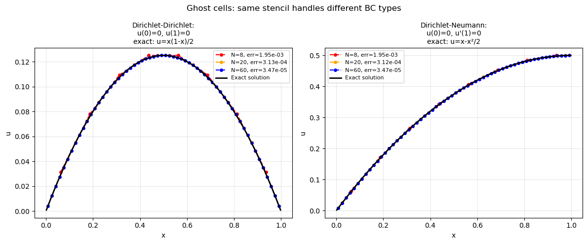
With ghost cells, the interior stencil (u[i+1]-2*u[i]+u[i-1]) applies at every point including the boundary — no special cases needed.

# ── Ghost cell demonstration ─────────────────────────────────────────────────
# Solve BVP: -d²u/dx² = 1 on [0,1]
# Three BC combinations:
#  (a) u(0)=0, u(1)=0  → Dirichlet-Dirichlet   → exact: u = x(1-x)/2
#  (b) u(0)=0, du/dx(1)=0  → Dirichlet-Neumann → exact: u = x - x²/2

def solve_1d_bvp(N, bc='dirichlet_dirichlet'):
    """
    Solve -d²u/dx² = 1 on [0,1].
    Uses the standard central-difference stencil.
    BCs implemented via a tridiagonal matrix (no ghost cells needed for this form,
    but the ghost-cell interpretation is shown in comments).
    """
    dx    = 1.0 / N
    x     = np.linspace(dx/2, 1 - dx/2, N)   # cell centres
    diag  =  2 * np.ones(N)
    off   = -1 * np.ones(N-1)
    rhs   = dx**2 * np.ones(N)

    if bc == 'dirichlet_dirichlet':
        # u(0)=0: ghost u[-1] = -u[0]  →  left-boundary row: 2u[0] - u[-1] - u[1] = dx²
        #                                 → 3u[0] - u[1] = dx² (after subst.)
        diag[0] = 3.0          # extra 1 on diagonal from ghost: -u[-1] = +u[0]
        # u(1)=0: ghost u[N] = -u[N-1]  → symmetric
        diag[-1] = 3.0
        exact = lambda xi: xi * (1 - xi) / 2

    elif bc == 'dirichlet_neumann':
        # Left: u(0)=0  → same as above
        diag[0]  = 3.0
        # Right: du/dx(1) = 0  → ghost u[N] = u[N-1]  → -u[N-1]+2u[N-1]-u[N-2]=dx²
        #                        →  u[N-1] - u[N-2] = dx²
        diag[-1] = 1.0         # only one neighbour contributes
        exact = lambda xi: xi - xi**2/2

    A = np.diag(diag) + np.diag(off, k=1) + np.diag(off, k=-1)
    u = np.linalg.solve(A, rhs)
    return x, u, exact(x)

fig, axes = plt.subplots(1, 2, figsize=(12, 5))

for ax, bc, title in zip(axes,
    ['dirichlet_dirichlet', 'dirichlet_neumann'],
    ['Dirichlet-Dirichlet:\nu(0)=0, u(1)=0\nexact: u=x(1-x)/2',
     'Dirichlet-Neumann:\nu(0)=0, u\'(1)=0\nexact: u=x-x²/2']):

    for N, color in zip([8, 20, 60], ['red', 'orange', 'blue']):
        x, u_num, u_ex = solve_1d_bvp(N, bc)
        ax.plot(x, u_num, 'o--', color=color, markersize=4,
                label=f'N={N}, err={np.max(np.abs(u_num-u_ex)):.2e}')

    x_fine = np.linspace(0, 1, 300)
    _, _, u_fine = solve_1d_bvp(300, bc)
    ax.plot(np.linspace(1/600, 1-1/600, 300), u_fine, 'k-', lw=2, label='Exact solution')
    ax.set_xlabel('x'); ax.set_ylabel('u')
    ax.set_title(title, fontsize=10)
    ax.legend(fontsize=8); ax.grid(True, alpha=0.3)

plt.suptitle('Ghost cells: same stencil handles different BC types', fontsize=12)
plt.tight_layout()
plt.show()

Summary

Formula	Name	Derivation	Error
$(u_{i+1}-u_i)/\Delta x$	Forward	(A) truncated	$O(\Delta x)$
$(u_i-u_{i-1})/\Delta x$	Backward	(B) truncated	$O(\Delta x)$
$(u_{i+1}-u_{i-1})/(2\Delta x)$	Central 1st	(A)−(B)	$O(\Delta x^2)$
$(u_{i+1}-2u_i+u_{i-1})/\Delta x^2$	Central 2nd	(A)+(B)	$O(\Delta x^2)$

Rules to live by:

Use central differences for diffusion terms (2nd derivative)
Use upwind differences for convection terms (1st derivative, direction matters)
Never use $\Delta x < 10^{-6}$ in double precision — round-off takes over
Ghost cells apply any BC to any interior stencil without special cases
Order of accuracy: halve $\Delta x$ → error drops by $2^p$ where $p$ is the order

Next: Module 1.6 — 1D Linear Advection: your first complete PDE solver, and the CFL condition that controls stability.

Exercise

Predict first, then verify.

Derive the fourth-order central difference for $du/dx$ using four neighbours. Start from Taylor expansions of $u_{i+2}$ , $u_{i+1}$ , $u_{i-1}$ , $u_{i-2}$ and find coefficients $a, b, c, d$ such that $u'_i \approx (a\,u_{i+2} + b\,u_{i+1} + c\,u_{i-1} + d\,u_{i-2})/\Delta x + O(\Delta x^4)$ .
Implement it and confirm on a convergence plot that the error slope is 4 (not 2).
At what $\Delta x$ does round-off overtake the 4th-order truncation error? Is this consistent with the formula $\Delta x^* \approx \epsilon_m^{1/(p+1)}$ ?