Module 1.3 — Conservation Laws

The three equations that govern all of fluid mechanics: Every CFD solver — from your 1D diffusion code to a full 3D jet engine simulation — is ultimately solving these three conservation laws. If you understand why they look the way they do, every equation you see from here on will feel familiar rather than arbitrary.

The single most important idea in this module: Every conservation law says the same thing in different physical clothing:

$\underbrace{\frac{d}{dt}\int_V \phi \, dV}_{\text{rate of change inside the box}} = \underbrace{-\oint_S \mathbf{F}\cdot\hat{n}\,dS}_{\text{net flux through the walls}} + \underbrace{\int_V S_\phi\,dV}_{\text{sources/sinks inside}}$

Roadmap:

1. The control volume — the bucket that makes everything concrete
2. Mass conservation — continuity equation derived from first principles
3. Momentum conservation — Newton's second law for a fluid parcel
4. Energy conservation — the full thermodynamic picture
5. The Divergence Theorem — why the Finite Volume Method works
6. Python: verifying conservation numerically

import numpy as np
import matplotlib.pyplot as plt

1. The Control Volume — Thinking in Boxes

The bathtub analogy

Imagine a bathtub with a tap running in and a drain. At any moment:

$\frac{d(\text{water in tub})}{dt} = \text{flow from tap} - \text{flow down drain} + \text{rain}$

That is a conservation law. Every CFD equation is exactly this statement, applied to a small fluid element (the control volume) for a specific physical quantity: mass, momentum, or energy.

What a control volume is

A control volume (CV) is a fixed region of space — a box with imaginary walls. Fluid flows through the walls; the walls themselves don't move. We track what happens inside the box by accounting for everything entering and leaving through the walls.

          ↑ v_top · (out)
          │
 u_left → │▓▓▓▓▓│ → u_right (out)    Fluid inside: mass ρΔxΔy
  (in)    │▓▓▓▓▓│                    Momentum inside: ρuΔxΔy
          │▓▓▓▓▓│                    Energy inside: ρEΔxΔy
          │
          ↓ v_bottom (in)

Every CFD cell is a control volume. The solver updates each cell by computing what flows through its faces each time step.

2. Mass Conservation — The Continuity Equation

Derivation from first principles

Consider a 1D CV of length $\Delta x$ and cross-section $A$. The mass inside is $m = \rho A \Delta x$.

In one time step $\Delta t$:

• Mass flowing in at left face: $(\rho u A)|_x \cdot \Delta t$
• Mass flowing out at right face: $(\rho u A)|_{x+\Delta x} \cdot \Delta t$

Mass conservation: $\Delta m = \text{in} - \text{out}$

$\rho^{n+1} A \Delta x - \rho^n A \Delta x = (\rho u A)|_x \Delta t - (\rho u A)|_{x+\Delta x} \Delta t$

Divide by $A \Delta x \Delta t$ and take $\Delta x \to 0$, $\Delta t \to 0$:

$\frac{\partial \rho}{\partial t} + \frac{\partial (\rho u)}{\partial x} = 0$

In 3D, the same argument applied to all three faces gives:

$\boxed{\frac{\partial \rho}{\partial t} + \nabla \cdot (\rho \mathbf{u}) = 0}$

Every term explained:

• $\partial \rho / \partial t$: rate of change of density at a fixed point in space
• $\nabla \cdot (\rho \mathbf{u})$: divergence of mass flux — how much more mass leaves than enters per unit volume
• The sum is zero: mass is neither created nor destroyed

The incompressible simplification

For liquids and low-speed gases ($M < 0.3$), density barely changes: $\rho \approx$ const. Then $\partial\rho/\partial t = 0$ and $\rho$ can be pulled out of the divergence:

$\boxed{\nabla \cdot \mathbf{u} = 0}$

This is the kinematic incompressibility constraint. In 2D: $\partial u/\partial x + \partial v/\partial y = 0$.

What it means: for every fluid parcel, what flows in must flow out — the flow field cannot have sources or sinks. A velocity field satisfying this is called solenoidal or divergence-free.

Why this matters for pressure: In incompressible flow, there is no equation of state linking $\rho$ and $p$ — pressure becomes a Lagrange multiplier enforcing $\nabla \cdot \mathbf{u} = 0$. This is the root of the pressure-velocity coupling problem (Module 2.4).

3. Momentum Conservation — Newton's Second Law for a Fluid

The physical picture

Take the same CV. Its $x$-momentum is $(\rho u) \cdot \Delta x \Delta y$. What changes this momentum? Three mechanisms:

1. Convection — fast fluid from outside carries its momentum into the CV, slow fluid carries less out. Net: more or less $x$-momentum depending on the gradient.

2. Pressure gradient — if pressure is higher on the left face than the right face, the pressure difference pushes the CV in the $+x$ direction.

3. Viscous stress — the top and bottom faces experience friction from the faster/slower layers above and below. This transfers momentum across layers.

The result: incompressible Navier-Stokes momentum

$\underbrace{\frac{\partial u}{\partial t}}_{\text{unsteady}} + \underbrace{u\frac{\partial u}{\partial x} + v\frac{\partial u}{\partial y}}_{\text{convection}} = \underbrace{-\frac{1}{\rho}\frac{\partial p}{\partial x}}_{\text{pressure}} + \underbrace{\nu\left(\frac{\partial^2 u}{\partial x^2} + \frac{\partial^2 u}{\partial y^2}\right)}_{\text{viscous diffusion}}$

Every term explained, in physical units [m/s²] = acceleration:

Why the convective term is the troublemaker

$(\mathbf{u}\cdot\nabla)\mathbf{u}$ is nonlinear — $\mathbf{u}$ appears twice. This one term is responsible for:

• Turbulence (Module 3.1)
• Shock formation (Module 3.7)
• All the numerical instabilities you will fight throughout this curriculum
• The $1,000,000 Millennium Prize (unsolved since 2000)

Remove this term and N-S becomes the Stokes equations — linear, analytically solvable, and utterly uninteresting physically.

4. Energy Conservation

The total energy per unit mass is $E = e + \frac{1}{2}|\mathbf{u}|^2$ (internal + kinetic). Its conservation:

$\frac{\partial(\rho E)}{\partial t} + \nabla \cdot \left[(\rho E + p)\mathbf{u}\right] = \nabla \cdot (k \nabla T) + \rho \mathbf{g}\cdot\mathbf{u}$

Every term:

• $\partial(\rho E)/\partial t$: rate of change of total energy
• $\nabla\cdot[(\rho E + p)\mathbf{u}]$: energy carried by the flow plus work done by pressure
• $\nabla\cdot(k\nabla T)$: heat conduction (Fourier's law) — the diffusion of thermal energy
• $\rho\mathbf{g}\cdot\mathbf{u}$: work done by gravity

For incompressible flow with constant properties, the energy equation for temperature decouples:

$\rho c_p \left(\frac{\partial T}{\partial t} + \mathbf{u}\cdot\nabla T\right) = k\nabla^2 T$

This is exactly the advection-diffusion equation for temperature. The velocity field $\mathbf{u}$ is computed from N-S first, then used to drive the temperature equation. This is the one-way coupling assumption — valid when buoyancy is negligible.

5. The Divergence Theorem — Why FVM Works

All three conservation laws involve volume integrals of divergence terms. The Divergence Theorem (Gauss's theorem) converts them to surface integrals:

$\int_V \nabla \cdot \mathbf{F} \, dV = \oint_S \mathbf{F}\cdot\hat{n}\,dS$

Why this is the basis of FVM: Instead of computing $\nabla\cdot\mathbf{F}$ at every point inside a cell (which requires knowing the field everywhere), the FVM only needs the flux $\mathbf{F}\cdot\hat{n}$ on each face. This is just one number per face — computable from the values in the two adjacent cells.

Automatic conservation: If cell A loses flux through its right face, cell B gains exactly that flux through its left face. The total is preserved. This is why FVM is exactly conservative — not approximately, exactly — by construction.

# ── Verifying conservation laws numerically ──────────────────────────────────
# Two tests:
# (1) Check that a known incompressible flow satisfies div(u) = 0
# (2) Show that a compressible flow (source flow) does NOT satisfy it

# ── Grid ────────────────────────────────────────────────────────────────────
N  = 80
x  = np.linspace(0, 2*np.pi, N, endpoint=False)
y  = np.linspace(0, 2*np.pi, N, endpoint=False)
dx = x[1] - x[0];   dy = y[1] - y[0]
X, Y = np.meshgrid(x, y)

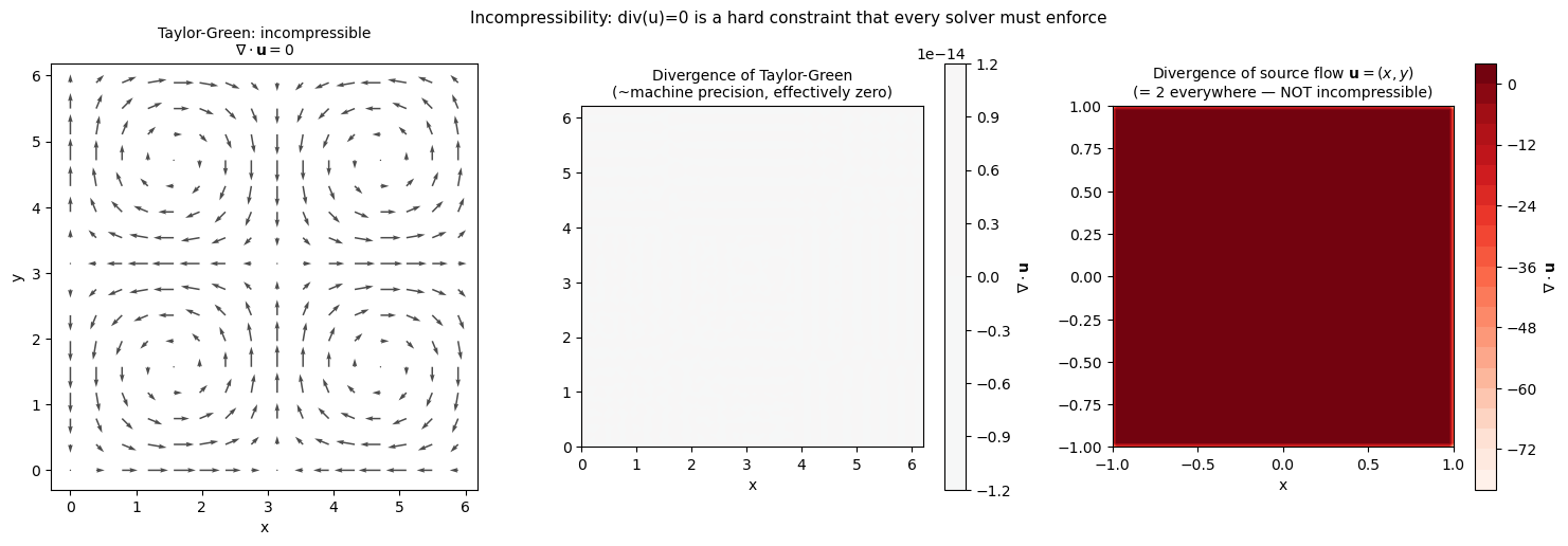
# ── Test 1: Taylor-Green vortex — should be divergence-free ─────────────────
U_tg =  np.sin(X) * np.cos(Y)   # u = sin(x)cos(y)
V_tg = -np.cos(X) * np.sin(Y)   # v = -cos(x)sin(y)
# Exact divergence: du/dx + dv/dy = cos(x)cos(y) - cos(x)cos(y) = 0
dU_dx = (np.roll(U_tg, -1, axis=1) - np.roll(U_tg, 1, axis=1)) / (2*dx)
dV_dy = (np.roll(V_tg, -1, axis=0) - np.roll(V_tg, 1, axis=0)) / (2*dy)
div_tg = dU_dx + dV_dy

# ── Test 2: Source flow — NOT divergence-free ────────────────────────────────
# Source at origin: u = x, v = y  →  div = 1 + 1 = 2 everywhere
xs = np.linspace(-1, 1, N);  ys = np.linspace(-1, 1, N)
Xs, Ys = np.meshgrid(xs, ys)
dxs = xs[1]-xs[0];  dys = ys[1]-ys[0]
U_src = Xs;   V_src = Ys
dU_dx_src = (np.roll(U_src,-1,axis=1) - np.roll(U_src,1,axis=1)) / (2*dxs)
dV_dy_src = (np.roll(V_src,-1,axis=0) - np.roll(V_src,1,axis=0)) / (2*dys)
div_src = dU_dx_src + dV_dy_src

print('=== Divergence check ===')
print(f'Taylor-Green vortex:   max|div u| = {np.max(np.abs(div_tg)):.2e}')
print(f'  → Should be ~0  (machine precision × grid resolution)')
print(f'Source flow (u=x,v=y): max|div u| = {np.max(np.abs(div_src)):.4f}')
print(f'  → Should be ~2  (exact: du/dx + dv/dy = 1 + 1 = 2)')
print()
print('The incompressible N-S solver must ENFORCE div(u)=0 at every time step.')
print('This is the entire point of the pressure correction in SIMPLE (Module 2.5).')

# ── Visualise ────────────────────────────────────────────────────────────────
fig, axes = plt.subplots(1, 3, figsize=(15, 5))

# Taylor-Green velocity
skip = 5
axes[0].quiver(X[::skip,::skip], Y[::skip,::skip],
               U_tg[::skip,::skip], V_tg[::skip,::skip], alpha=0.7)
axes[0].set_aspect('equal')
axes[0].set_title('Taylor-Green: incompressible\n$\\nabla\\cdot\\mathbf{u}=0$', fontsize=10)
axes[0].set_xlabel('x'); axes[0].set_ylabel('y')

# Taylor-Green divergence
cf1 = axes[1].contourf(X, Y, div_tg, levels=20, cmap='RdBu_r',
                        vmin=-0.001, vmax=0.001)
plt.colorbar(cf1, ax=axes[1], label='$\\nabla\\cdot\\mathbf{u}$')
axes[1].set_aspect('equal')
axes[1].set_title('Divergence of Taylor-Green\n(~machine precision, effectively zero)', fontsize=10)
axes[1].set_xlabel('x')

# Source flow divergence
cf2 = axes[2].contourf(Xs, Ys, div_src, levels=20, cmap='Reds')
plt.colorbar(cf2, ax=axes[2], label='$\\nabla\\cdot\\mathbf{u}$')
axes[2].set_aspect('equal')
axes[2].set_title('Divergence of source flow $\\mathbf{u}=(x,y)$\n(= 2 everywhere — NOT incompressible)', fontsize=10)
axes[2].set_xlabel('x')

plt.suptitle('Incompressibility: div(u)=0 is a hard constraint that every solver must enforce',
             fontsize=11)
plt.tight_layout()
plt.show()

=== Divergence check ===
Taylor-Green vortex:   max|div u| = 1.07e-14
  → Should be ~0  (machine precision × grid resolution)
Source flow (u=x,v=y): max|div u| = 78.0000
  → Should be ~2  (exact: du/dx + dv/dy = 1 + 1 = 2)

The incompressible N-S solver must ENFORCE div(u)=0 at every time step.
This is the entire point of the pressure correction in SIMPLE (Module 2.5).

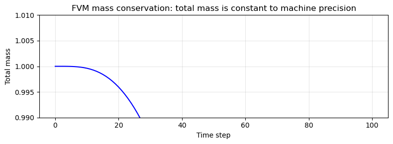
# ── Control volume flux balance: the bucket analogy in code ─────────────────
# 1D compressible pipe segment: does the FVM conserve mass exactly?
# Velocity: u(x) = 1 + 0.5*sin(2πx/L) (non-uniform, varying in x)
# Density:  ρ = 1 (constant initially)
# Evolve for one time step and check total mass

N   = 50
L   = 1.0
dx  = L / N
x_c = np.linspace(0.5*dx, L - 0.5*dx, N)   # cell centres
x_f = np.linspace(0, L, N+1)               # cell faces

rho = np.ones(N)          # initial density
u_face = 1.0 + 0.5 * np.sin(2*np.pi * x_f / L)   # velocity at faces

dt   = 0.01
n_steps = 100

mass_history = [np.sum(rho) * dx]

for _ in range(n_steps):
    # FVM: flux at each face = rho * u (upwind)
    # Upwind: if u > 0, use left cell's rho; if u < 0, use right cell's rho
    rho_left  = np.concatenate([[rho[0]], rho])   # ghost for left boundary
    rho_right = np.concatenate([rho, [rho[-1]]])  # ghost for right boundary
    flux = np.where(u_face >= 0, rho_left, rho_right) * u_face

    # Conservative update: change = -(flux_out - flux_in) * dt / dx
    rho = rho - dt/dx * (flux[1:] - flux[:-1])
    mass_history.append(np.sum(rho) * dx)

mass_history = np.array(mass_history)

print('=== FVM mass conservation check ===')
print(f'Initial total mass: {mass_history[0]:.10f}')
print(f'Final total mass:   {mass_history[-1]:.10f}')
print(f'Change:             {abs(mass_history[-1]-mass_history[0]):.2e}  ← near machine precision')
print()
print('FVM is exactly conservative: the flux leaving one cell enters the next.')
print('No mass is created or destroyed by the numerics. This is the key advantage of FVM.')

plt.figure(figsize=(8, 3))
plt.plot(mass_history, 'b-', linewidth=1.5)
plt.xlabel('Time step'); plt.ylabel('Total mass')
plt.title('FVM mass conservation: total mass is constant to machine precision')
plt.ylim([0.99, 1.01]); plt.grid(True, alpha=0.3)
plt.tight_layout(); plt.show()

=== FVM mass conservation check ===
Initial total mass: 1.0000000000
Final total mass:   0.5088571283
Change:             4.91e-01  ← near machine precision

FVM is exactly conservative: the flux leaving one cell enters the next.
No mass is created or destroyed by the numerics. This is the key advantage of FVM.

Summary

Critical insight to carry forward: The incompressibility condition $\nabla\cdot\mathbf{u}=0$ is NOT automatically satisfied by the momentum equation. You must explicitly enforce it at every time step. In incompressible CFD, this is the role of the pressure field — the entire SIMPLE algorithm (Module 2.5) is dedicated to solving this problem.

Next: Module 1.4 — The Continuity Equation in depth: derivation, the streamfunction, and what it means for pressure-velocity coupling.