1D Linear Advection
Lesson 1.6 of the CFD for Absolute Beginners course — 1D Linear Advection.
Module 1.6 — 1D Linear Advection
Why start here? The linear advection equation is the simplest non-trivial PDE. It has an exact solution so you can measure your numerical error precisely. It exposes every major issue in CFD — stability, accuracy, diffusion error, dispersion error — in a setting simple enough to understand them completely before moving to Navier-Stokes.
The equation:
A scalar quantity (temperature, dye concentration, or a wave) transported at constant speed without deforming. The exact solution is pure translation: .
Roadmap:
- Physical intuition — what the equation actually describes
- Discretisation — the four main schemes
- The CFL condition — the most important stability criterion in CFD
- Numerical diffusion and dispersion — why your wave smears or wiggles
- Modified equation analysis — what equation the scheme actually solves
- Implementation and comparison of all four schemes
import numpy as np
import matplotlib.pyplot as plt
1. Physical Intuition — The Conveyor Belt
The analogy
Imagine a conveyor belt moving at constant speed to the right. You place a dye blob on it. The blob moves to the right at speed . It does not spread, shrink, or change shape — it is simply translated.
That is linear advection. The blob's shape is at . At time , it is at .
Why this is the hardest equation to solve numerically
The exact solution is a rigid translation. The numerical solution should be exactly the same. But:
- Upwind scheme: smooths the blob over time (artificial diffusion)
- Central scheme: adds oscillations that weren't there (artificial dispersion)
- Lax-Friedrichs: very diffusive — the blob melts away
- Lax-Wendroff: second-order accurate but wiggles behind sharp features
None of them is perfect. This tension — diffusion vs. dispersion — is the central design trade-off in CFD numerics.
2. The Schemes — Four Approaches to Discretising
All use forward Euler time stepping:
The difference is in how the flux is computed:
FTBS — Forward Time, Backward Space (upwind for ): where is the CFL number. Uses the upstream cell — stable but diffusive.
FTCS — Forward Time, Central Space: Second-order in space but unconditionally unstable. Never use it for pure advection.
Lax-Friedrichs: Stable for but replaces with the average of neighbours — very diffusive.
Lax-Wendroff: Second-order in both space and time. Stable for . Dispersive — oscillates near discontinuities.
3. The CFL Condition — Why It Is the Most Important Number in CFD
Physical interpretation
The CFL number is:
If : the wave travels more than one cell per time step. The stencil does not contain the information needed to correctly propagate the wave — the wave has "jumped over" the stencil. Result: the scheme becomes unstable and the solution blows up exponentially.
If : the wave moves at most one cell per step. The stencil contains all the information needed.
If : For the upwind scheme, the solution is exact — the wave translates by exactly one cell, matching the exact shift .
The CFL condition for common schemes
| Scheme | Stability condition |
|---|---|
| Upwind (FTBS) | |
| FTCS | Unconditionally unstable (any ) |
| Lax-Friedrichs | |
| Lax-Wendroff |
In 2D: the combined CFL condition
This will appear every time you set the time step in Modules 2–4.
# ── Complete solver with all four schemes ────────────────────────────────────
def advect_1d(u0, c, dx, dt, nt, scheme='upwind'):
"""1D linear advection with periodic BCs."""
u = u0.copy()
nu = c * dt / dx # CFL number
for _ in range(nt):
un = u.copy() # must save old values before update
if scheme == 'upwind':
# FTBS: backward difference (upwind for c>0)
u[1:] = un[1:] - nu * (un[1:] - un[:-1])
u[0] = un[0] - nu * (un[0] - un[-1]) # periodic BC
elif scheme == 'ftcs':
# FTCS: central space — UNSTABLE, shown for illustration only
u[1:-1] = un[1:-1] - nu/2 * (un[2:] - un[:-2])
u[0] = un[0] - nu/2 * (un[1] - un[-1])
u[-1] = un[-1] - nu/2 * (un[0] - un[-2])
elif scheme == 'lax_friedrichs':
# Stable but very diffusive: averages neighbours first
u[1:-1] = 0.5*(un[2:]+un[:-2]) - nu/2*(un[2:]-un[:-2])
u[0] = 0.5*(un[1] +un[-1] ) - nu/2*(un[1] -un[-1] )
u[-1] = u[0]
elif scheme == 'lax_wendroff':
# Second-order in space and time, dispersive near shocks
u[1:-1] = (un[1:-1]
- nu/2 * (un[2:] - un[:-2])
+ nu**2/2 * (un[2:] - 2*un[1:-1] + un[:-2]))
u[0] = (un[0]
- nu/2 * (un[1] - un[-1])
+ nu**2/2 * (un[1] - 2*un[0] + un[-1]))
u[-1] = u[0]
return u
# ── Setup ────────────────────────────────────────────────────────────────────
N = 120
L = 2.0
dx = L / N
x = np.linspace(0, L, N, endpoint=False)
c = 1.0
cfl = 0.7 # CFL number
dt = cfl * dx / c
T = 1.2 # simulate until t=1.2
nt = int(T / dt)
# ── Initial condition: mixed test — step (discontinuity) + Gaussian (smooth) ─
u0 = np.zeros(N)
u0[(x > 0.2) & (x < 0.5)] = 1.0 # step — hard test
u0 += 0.8 * np.exp(-((x - 1.2)**2) / 0.015) # Gaussian — smooth test
# ── Exact solution: shift by c*T (modulo L for periodic domain) ──────────────
x_shifted = (x - c*T) % L
u_exact = np.zeros(N)
u_exact[(x_shifted > 0.2) & (x_shifted < 0.5)] = 1.0
u_exact += 0.8 * np.exp(-((x_shifted - 1.2)**2) / 0.015)
schemes = ['upwind', 'lax_friedrichs', 'lax_wendroff']
colors = ['royalblue', 'darkorange', 'green']
results = {s: advect_1d(u0, c, dx, dt, nt, s) for s in schemes}
fig, axes = plt.subplots(1, 3, figsize=(15, 5))
for ax, scheme, color in zip(axes, schemes, colors):
u_num = results[scheme]
l2 = np.sqrt(np.mean((u_num - u_exact)**2))
ax.plot(x, u0, 'k--', lw=1.2, alpha=0.4, label='Initial $t=0$')
ax.plot(x, u_exact, 'k-', lw=2, label='Exact $t=1.2$')
ax.plot(x, u_num, '-', lw=1.8, color=color, label=f'{scheme.replace("_"," ").title()}')
ax.set_title(f'{scheme.replace("_"," ").title()}\nL2 error = {l2:.4f}', fontsize=10)
ax.set_xlabel('x'); ax.set_ylabel('u')
ax.legend(fontsize=8); ax.set_ylim(-0.4, 1.5)
ax.grid(True, alpha=0.3)
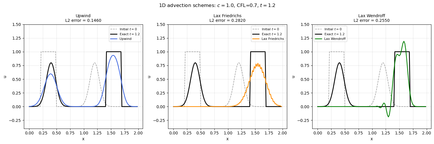
plt.suptitle(f'1D advection schemes: $c={c}$, CFL={cfl}, $t={T}$', fontsize=12)
plt.tight_layout()
plt.show()
print('Observations:')
print(' Upwind: diffusive — step has rounded edges, Gaussian is smeared')
print(' Lax-Friedrichs: very diffusive — even worse than upwind (replaces uᵢ with neighbour average)')
print(' Lax-Wendroff: dispersive — wiggles behind the step, but Gaussian is sharper')
Observations:
  Upwind:        diffusive — step has rounded edges, Gaussian is smeared
  Lax-Friedrichs: very diffusive — even worse than upwind (replaces uᵢ with neighbour average)
  Lax-Wendroff:  dispersive — wiggles behind the step, but Gaussian is sharper
4. Modified Equation Analysis — What Equation Does the Scheme Actually Solve?
The surprising truth about numerical diffusion
The upwind scheme does not solve exactly. By substituting Taylor expansions into the scheme and re-expanding, you can show that it actually solves:
The upwind scheme adds artificial diffusion with coefficient .
Key insight: the numerical diffusion vanishes as (consistent scheme), but for any finite grid it smooths sharp features. This is why the upwind scheme smears the step discontinuity.
At CFL = 1: — the upwind scheme is exact! This is why the advection test at always gives perfect results for upwind.
Similarly, Lax-Wendroff adds artificial dispersion (fourth-order derivative term), which causes the trailing oscillations you see near the step.
The fundamental trade-off:
- Diffusion damps all wave components equally → blurs features
- Dispersion makes different frequencies travel at different speeds → wiggles
- TVD schemes (Module 3.4) adapt between the two based on local gradient, giving the best of both worlds
# ── CFL instability demonstration ───────────────────────────────────────────
# Show what happens when CFL > 1 with the upwind scheme
N = 80
dx = 2.0 / N
x = np.linspace(0, 2, N, endpoint=False)
c = 1.0
u_init = np.exp(-((x-0.5)**2)/0.02) # Gaussian blob
fig, axes = plt.subplots(1, 3, figsize=(14, 4))
for ax, cfl_val in zip(axes, [0.5, 1.0, 1.5]):
dt_val = cfl_val * dx / c
u = u_init.copy()
blown = False
for step in range(60):
un = u.copy()
u[1:] = un[1:] - cfl_val * (un[1:] - un[:-1])
u[0] = un[0] - cfl_val * (un[0] - un[-1])
if np.max(np.abs(u)) > 5:
blown = True
break
ax.plot(x, u_init, 'k--', lw=1.5, alpha=0.5, label='Initial')
ax.plot(x, u, 'r-' if blown else 'b-', lw=1.8)
status = '💥 UNSTABLE — blows up' if blown else '✓ Stable'
ax.set_title(f'CFL = {cfl_val} → {status}', fontsize=10)
ax.set_xlabel('x'); ax.set_ylabel('u')
ax.set_ylim(-2, 2); ax.grid(True, alpha=0.3)
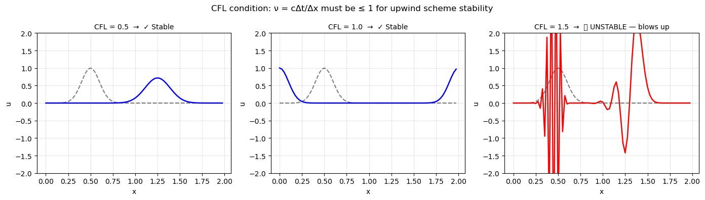
plt.suptitle('CFL condition: ν = cΔt/Δx must be ≤ 1 for upwind scheme stability', fontsize=12)
plt.tight_layout()
plt.show()
print('CFL = 0.5: stable, Gaussian moves and stays bounded')
print('CFL = 1.0: stable, exact at CFL=1 for upwind (zero numerical diffusion)')
print('CFL = 1.5: unstable — wave travels 1.5 cells per step,')
print(' jumping past the stencil, error grows exponentially')
/var/folders/j6/slfvk4c54yj6lt99pq5rjh8m0000gn/T/ipykernel_6926/3626125202.py:35: UserWarning: Glyph 128165 (\N{COLLISION SYMBOL}) missing from font(s) DejaVu Sans.
  plt.tight_layout()
/Volumes/Storage/miniconda3/lib/python3.13/site-packages/IPython/core/pylabtools.py:170: UserWarning: Glyph 128165 (\N{COLLISION SYMBOL}) missing from font(s) DejaVu Sans.
  fig.canvas.print_figure(bytes_io, **kw)
CFL = 0.5: stable, Gaussian moves and stays bounded
CFL = 1.0: stable, exact at CFL=1 for upwind (zero numerical diffusion)
CFL = 1.5: unstable — wave travels 1.5 cells per step,
           jumping past the stencil, error grows exponentially
Summary
| Scheme | Stability | Order (space×time) | Error character |
|---|---|---|---|
| Upwind (FTBS) | 1×1 | Diffusive — smears features | |
| FTCS (central) | Unconditionally unstable | 2×1 | Always blows up |
| Lax-Friedrichs | 1×1 | Very diffusive | |
| Lax-Wendroff | 2×2 | Dispersive — oscillates near shocks |
The CFL condition is the single most important criterion in explicit CFD. It says: your time step must be small enough that the wave travels at most one cell. Violate it once and the solution immediately diverges.
In every solver you write, compute as:
dt = cfl * dx / max_speed # set cfl=0.5–0.9 for safety
Next: Module 1.7 — 1D Diffusion Equation: implicit vs. explicit time-stepping, and why one scheme needs 100× fewer time steps than the other.
Exercise
Predict first, then code.
-
At CFL = 1, the upwind scheme is exact. Verify this: run the step-function IC with for 50 steps. Does the solution match the exact translation? Why does this happen? (Hint: look at what
u[1:] = un[1:] - 1.0*(un[1:] - un[:-1])simplifies to when .) -
The modified equation for Lax-Wendroff has a dispersive term proportional to . Given a sine wave : does the numerical speed of this wave () increase or decrease with wavenumber ? Higher-frequency components travel faster or slower than lower-frequency ones?
-
Implement a scheme that switches between upwind and Lax-Wendroff based on the local gradient ratio : use Lax-Wendroff where (smooth region) and upwind where (near extrema). This is the Minmod flux-limited scheme — a preview of Module 3.4.