2D Scalar Transport
Lesson 2.1 of the CFD for Absolute Beginners course — 2D Scalar Transport.
Lesson 2.1 — 2D Scalar Transport
From 1D to 2D: Adding a Second Dimension
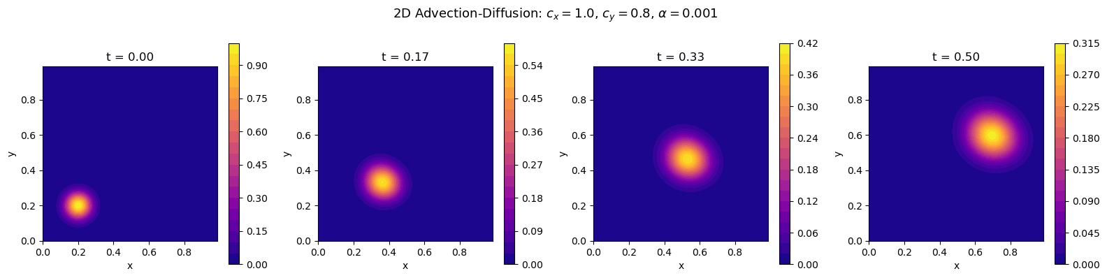
Imagine dropping a dye blob into a river that flows diagonally. The blob drifts with the current (advection in both and ) and simultaneously spreads outward (diffusion in both directions). The 2D advection-diffusion equation describes this:
Everything from Module 1 generalises directly — just apply the same 1D stencils in each spatial direction. The only new complexity is the 2D array indexing and boundary conditions on all four sides.
2D Grid and Indexing Convention
The standard convention in this curriculum:
u[j, i]  →  position (x_i, y_j)
j = row index    → y direction  (axis 0)
i = column index → x direction  (axis 1)
Stencil in 2D:
- Right neighbour:
u[j, i+1]→u[j, 2:] - Left neighbour:
u[j, i-1]→u[j, :-2] - Top neighbour:
u[j+1, i]→u[2:, j]→u[2:, :] - Bottom neighbour:
u[j-1, i]→u[:-2, :]
CFL Condition in 2D
The 2D CFL condition requires stability in each direction:
In practice, use:
Operator Splitting (Strang Splitting)
A clean way to extend 1D schemes to 2D: solve each direction separately in alternating half-steps.
This is Strang splitting — second-order accurate despite using 1D solvers as building blocks. Used in many production CFD codes for operator simplicity.
import numpy as np
import matplotlib.pyplot as plt

# 2D advection-diffusion: explicit upwind + central diffusion

nx, ny = 80, 80
Lx, Ly = 1.0, 1.0
dx = Lx / nx
dy = Ly / ny
x  = np.linspace(0, Lx, nx, endpoint=False)
y  = np.linspace(0, Ly, ny, endpoint=False)
X, Y = np.meshgrid(x, y)

cx, cy = 1.0, 0.8  # advection velocities
alpha  = 1e-3       # diffusivity

# Stable time step
dt = 0.4 / (abs(cx)/dx + abs(cy)/dy + 2*alpha*(1/dx**2 + 1/dy**2))

# Initial condition: Gaussian blob at (0.2, 0.2)
u = np.exp(-((X - 0.2)**2 + (Y - 0.2)**2) / 0.005)

T  = 0.5
nt = int(T / dt)

# Snapshot times
snapshots = []
snap_times = [0, T/3, 2*T/3, T]
snap_steps = [int(t/dt) for t in snap_times]
step = 0

snapshots.append(u.copy())

for n in range(nt):
    u_old = u.copy()

    # Upwind advection in x
    u[1:-1, 1:-1] -= dt * cx/dx * (u_old[1:-1, 1:-1] - u_old[1:-1, :-2])
    # Upwind advection in y
    u[1:-1, 1:-1] -= dt * cy/dy * (u_old[1:-1, 1:-1] - u_old[:-2, 1:-1])
    # Diffusion: central
    u[1:-1, 1:-1] += dt * alpha * (
        (u_old[1:-1, 2:] - 2*u_old[1:-1, 1:-1] + u_old[1:-1, :-2]) / dx**2 +
        (u_old[2:, 1:-1] - 2*u_old[1:-1, 1:-1] + u_old[:-2, 1:-1]) / dy**2
    )
    # Periodic BCs
    u[0,  :] = u[-2, :]
    u[-1, :] = u[1,  :]
    u[:,  0] = u[:, -2]
    u[:, -1] = u[:,  1]

    step += 1
    if step in snap_steps[1:]:
        snapshots.append(u.copy())

fig, axes = plt.subplots(1, 4, figsize=(16, 4))
for ax, snap, t in zip(axes, snapshots, snap_times):
    cf = ax.contourf(X, Y, snap, levels=20, cmap='plasma', vmin=0)
    plt.colorbar(cf, ax=ax)
    ax.set_title(f't = {t:.2f}')
    ax.set_xlabel('x'); ax.set_ylabel('y')
    ax.set_aspect('equal')

plt.suptitle(f'2D Advection-Diffusion: $c_x={cx}$, $c_y={cy}$, $\\alpha={alpha}$', fontsize=13)
plt.tight_layout()
plt.show()

print(f"dt = {dt:.6f}  |  CFL_x = {cx*dt/dx:.3f}  |  CFL_y = {cy*dt/dy:.3f}")
dt = 0.002358 | CFL_x = 0.189 | CFL_y = 0.151
Boundary Conditions in 2D
| BC type | Description | Implementation |
|---|---|---|
| Dirichlet | Prescribed value at boundary | Set u[0,:] = value directly |
| Neumann | Prescribed gradient (e.g., zero flux) | u[0,:] = u[1,:] (zero gradient) |
| Periodic | Domain wraps around | u[0,:] = u[-2,:], u[-1,:] = u[1,:] |
| Outflow | Value advects out, no reflection | Upwind: extrapolate u[-1,:] = u[-2,:] |
Key Takeaways
- 2D transport is a direct extension of 1D — apply 1D stencils in each spatial direction.
- The 2D CFL condition combines the constraints from all directions.
- Operator splitting (Strang) achieves 2nd-order accuracy using 1D sweeps.
- Boundary conditions must be applied on all four sides — easy to miss in the code!
Next: Lesson 2.2 — Finite Volume Method: flux balance on control volumes.