Module 3: Advanced Topics · Lesson 7
Compressible Flow
Lesson 3.7 of the CFD for Absolute Beginners course — Compressible Flow.
Lesson 3.7 — Compressible Flow
When Density Changes Matter
All of Module 2 assumed const (incompressible). This breaks down when:
- Flow speed exceeds Mach 0.3 (, where is the speed of sound)
- Large temperature differences exist (heating/cooling changes density)
- Shocks are present (density jumps discontinuously across a shock)
For supersonic flow (), information cannot travel upstream — the pressure Poisson approach of Module 2 breaks down completely. We need a different formulation.
The Euler Equations (Inviscid Compressible Flow)
The compressible Euler equations in conservation form:
where the conserved vector and fluxes are:
\mathbf{F} = \begin{pmatrix}\rho u \\ \rho u^2 + p \\ \rho u v \\ (\rho E + p)u\end{pmatrix}, \quad \mathbf{G} = \begin{pmatrix}\rho v \\ \rho u v \\ \rho v^2 + p \\ (\rho E + p)v\end{pmatrix}$$ The pressure is closed by the **ideal gas equation of state**: $$p = (\gamma - 1)\left(\rho E - \frac{\rho(u^2 + v^2)}{2}\right)$$ with $\gamma = 1.4$ for air (ratio of specific heats). --- ## The Riemann Problem The key building block of compressible FVM is the **Riemann problem**: given two constant states $U_L$ and $U_R$ on either side of a cell face, what flux $F$ should we assign? The exact Riemann solver (Godunov, 1959) is expensive. Approximate Riemann solvers: - **Roe's solver**: linearizes the Jacobian at an average state — fast and accurate. - **HLLE/HLLC**: uses wave-speed estimates — simpler and more robust. - **Lax-Friedrichs**: simplest but most diffusive. --- ## Mach Number Regimes | Regime | Mach range | Characteristics | |--------|-----------|------------------| | Subsonic | $M < 0.3$ | Incompressible; ignore density changes | | Transonic | $0.3 < M < 1$ | Compressibility important; no shock (in open flow) | | Sonic | $M = 1$ | Flow choked at throat; shock formation threshold | | Supersonic | $M > 1$ | Oblique shocks; expansion fans; elliptic → hyperbolic | | Hypersonic | $M > 5$ | Extreme heating; real gas effects; ionisation | --- ## Normal Shock Relations Across a normal shock, Rankine-Hugoniot conditions give: $$\frac{\rho_2}{\rho_1} = \frac{(\gamma+1)M_1^2}{(\gamma-1)M_1^2 + 2}$$ $$\frac{p_2}{p_1} = \frac{2\gamma M_1^2 - (\gamma-1)}{\gamma+1}$$ $$M_2^2 = \frac{(\gamma-1)M_1^2 + 2}{2\gamma M_1^2 - (\gamma-1)}$$ The shock is a mathematical discontinuity — in numerical CFD, it smears over 2-5 cells depending on the scheme. ```python import numpy as np import matplotlib.pyplot as plt # 1D Euler equations: Sod shock tube test # Classic benchmark: left state (high p,rho) meets right state (low p,rho) gamma = 1.4 def primitives_to_conserved(rho, u, p): E = p/(gamma-1)/rho + 0.5*u**2 return np.array([rho, rho*u, rho*E]) def conserved_to_primitives(U): rho = U[0] u = U[1] / rho E = U[2] / rho p = (gamma - 1) * rho * (E - 0.5*u**2) return rho, u, p def euler_flux(U): rho, u, p = conserved_to_primitives(U) E = U[2] / rho return np.array([rho*u, rho*u**2 + p, (rho*E + p)*u]) def lax_friedrichs_flux(UL, UR, dx, dt): return 0.5*(euler_flux(UL) + euler_flux(UR)) - 0.5*(dx/dt)*(UR - UL) # Grid N = 200 L = 1.0 dx = L / N x = np.linspace(dx/2, L - dx/2, N) # Sod initial conditions U = np.zeros((3, N)) for i, xi in enumerate(x): if xi < 0.5: U[:, i] = primitives_to_conserved(1.0, 0.0, 1.0) # left: high pressure else: U[:, i] = primitives_to_conserved(0.125, 0.0, 0.1) # right: low pressure # Time march T = 0.2 t = 0.0 CFL = 0.4 while t < T: # Compute wave speeds for time step rho, u, p = conserved_to_primitives(U) a = np.sqrt(np.maximum(gamma * p / rho, 1e-10)) S_max = np.max(np.abs(u) + a) dt = CFL * dx / S_max dt = min(dt, T - t) # Fluxes at cell faces using Lax-Friedrichs F_faces = np.zeros((3, N+1)) # Left BC: zero-gradient F_faces[:, 0] = lax_friedrichs_flux(U[:, 0], U[:, 0], dx, dt) # Right BC F_faces[:, -1] = lax_friedrichs_flux(U[:, -1], U[:, -1], dx, dt) # Interior faces for i in range(1, N): F_faces[:, i] = lax_friedrichs_flux(U[:, i-1], U[:, i], dx, dt) # Update U -= dt/dx * (F_faces[:, 1:] - F_faces[:, :-1]) t += dt rho_f, u_f, p_f = conserved_to_primitives(U) # Exact Sod solution (simplified reference) # Using known positions of waves at t=0.2: # Rarefaction fan: x in [0.263, 0.486] # Contact discontinuity: x ~ 0.685 # Shock: x ~ 0.851 fig, axes = plt.subplots(1, 3, figsize=(14, 4)) labels = ['Density $\\rho$', 'Velocity $u$', 'Pressure $p$'] fields = [rho_f, u_f, p_f] for ax, field, label in zip(axes, fields, labels): ax.plot(x, field, 'b-', linewidth=2) ax.set_xlabel('x'); ax.set_ylabel(label) ax.set_title(f'Sod shock tube: {label} at t={T}') ax.grid(True, alpha=0.3) # Annotate wave structures ax.axvspan(0.26, 0.49, alpha=0.1, color='blue', label='Rarefaction fan') ax.axvline(0.69, color='green', linestyle='--', alpha=0.6, label='Contact') ax.axvline(0.85, color='red', linestyle='--', alpha=0.6, label='Shock') ax.legend(fontsize=7) plt.suptitle('Sod Shock Tube: 1D Euler equations (Lax-Friedrichs)', fontsize=13) plt.tight_layout() plt.show() ``` <div className="nb-figure"> 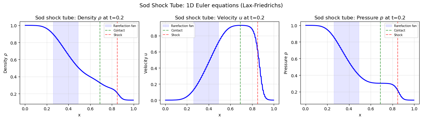 </div> ```python # Normal shock relations: properties across a shock gamma = 1.4 M1_range = np.linspace(1.0, 5.0, 200) # Density ratio rho_ratio = (gamma+1)*M1_range**2 / ((gamma-1)*M1_range**2 + 2) # Pressure ratio p_ratio = (2*gamma*M1_range**2 - (gamma-1)) / (gamma+1) # Downstream Mach M2 = np.sqrt(((gamma-1)*M1_range**2 + 2) / (2*gamma*M1_range**2 - (gamma-1))) # Total pressure ratio (entropy production) p0_ratio = (((gamma+1)*M1_range**2 / ((gamma-1)*M1_range**2 + 2))**(gamma/(gamma-1)) * ((gamma+1) / (2*gamma*M1_range**2 - (gamma-1)))**(1/(gamma-1))) fig, axes = plt.subplots(2, 2, figsize=(12, 8)) plots = [ (axes[0,0], M2, '$M_2$ (downstream Mach)', 'Tab:blue'), (axes[0,1], p_ratio, '$p_2/p_1$ (pressure jump)', 'Tab:red'), (axes[1,0], rho_ratio, '$\\rho_2/\\rho_1$ (density jump)', 'Tab:green'), (axes[1,1], p0_ratio, '$p_{02}/p_{01}$ (total pressure ratio)', 'Tab:purple'), ] for ax, field, label, color in plots: ax.plot(M1_range, field, color=color, linewidth=2) ax.set_xlabel('Upstream Mach number $M_1$') ax.set_ylabel(label) ax.set_title(label) ax.grid(True, alpha=0.3) ax.axvline(1.0, color='gray', linestyle='--', alpha=0.5) axes[1,1].set_ylim(0, 1.05) axes[1,1].axhline(1.0, color='gray', linestyle='--', alpha=0.5) plt.suptitle('Normal shock relations ($\\gamma = 1.4$, air)', fontsize=13) plt.tight_layout() plt.show() # Print some key values for M1 in [1.5, 2.0, 3.0, 5.0]: p_r = (2*gamma*M1**2 - (gamma-1)) / (gamma+1) rho_r = (gamma+1)*M1**2 / ((gamma-1)*M1**2 + 2) M2_v = np.sqrt(((gamma-1)*M1**2 + 2) / (2*gamma*M1**2 - (gamma-1))) print(f"M1={M1:.1f}: p2/p1={p_r:.2f}, rho2/rho1={rho_r:.2f}, M2={M2_v:.3f}") ``` <div className="nb-figure"> 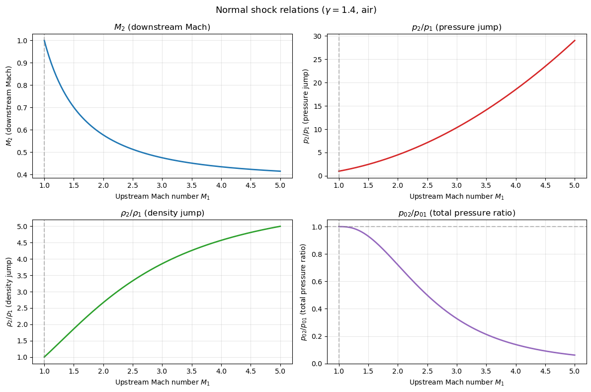 </div> <div className="nb-output"> ``` M1=1.5: p2/p1=2.46, rho2/rho1=1.86, M2=0.701 M1=2.0: p2/p1=4.50, rho2/rho1=2.67, M2=0.577 M1=3.0: p2/p1=10.33, rho2/rho1=3.86, M2=0.475 M1=5.0: p2/p1=29.00, rho2/rho1=5.00, M2=0.415 ``` </div> ## Key Takeaways - Compressible flow ($M > 0.3$): density changes, pressure waves travel at finite speed $c_s$. - Governing equations: conservation of mass, momentum, **energy** (all coupled through $\rho$). - Closed by ideal gas equation of state: $p = (\gamma-1)(\rho E - \frac{1}{2}\rho u^2)$. - Shocks are discontinuities captured numerically using approximate Riemann solvers (Roe, HLLC). - Normal shock: increases $p$, $\rho$, $T$; decreases $M$, total pressure (entropy production). - Sod shock tube is the standard 1D benchmark for compressible solvers. --- **Next**: Lesson 3.8 — Physics-Informed Neural Networks (PINNs): ML meets CFD.