Module 1.7 — 1D Diffusion Equation

The equation: $\frac{\partial u}{\partial t} = \alpha \frac{\partial^2 u}{\partial x^2}$

where $\alpha$ is the diffusivity — same equation, different physical interpretation depending on context:

Why this module is critical before SIMPLE: The viscous terms in the Navier-Stokes equations are diffusion terms ($\nu\nabla^2\mathbf{u}$). The stability of the momentum solver depends entirely on choosing the right time-stepping scheme for diffusion. This module explains why.

Roadmap:

1. Physical intuition — what diffusion actually does to a field
2. Explicit (FTCS) scheme — simple to code, severely limited
3. The diffusion stability condition — why it is much harsher than CFL
4. Implicit (BTCS) scheme — unconditionally stable, one tridiagonal solve
5. Crank-Nicolson — second-order accurate in time and space
6. Fourier stability analysis — prove stability from first principles
7. Comparison: when to use each scheme

import numpy as np
import matplotlib.pyplot as plt
from scipy.linalg import solve_banded

1. Physical Intuition — Why Diffusion Smooths Everything

The hot rod analogy

Hold a metal rod with one end in a flame. Heat flows from the hot end toward the cold end — not at a fixed wave speed like advection, but by smoothing out temperature gradients. A spike in temperature spreads outward and flattens. Sharp differences get erased over time.

Mathematically, the second derivative $\partial^2 T/\partial x^2$ tells you the concavity of the temperature profile:

• If $T$ is concave up (valley): $T'' > 0$ → temperature increases there
• If $T$ is concave down (peak): $T'' < 0$ → temperature decreases there

In plain English: peaks get shorter, valleys fill up. Diffusion is anti-curvature.

Exact solution by Fourier analysis

The exact solution for a single sine-wave initial condition $u(x,0) = \sin(kx)$ is:

$u(x,t) = \sin(kx) \cdot e^{-\alpha k^2 t}$

Two key observations:

1. High wavenumbers ($k$ large) decay exponentially faster — fine-scale features vanish quickly
2. The decay rate is $\alpha k^2$ — proportional to the square of the wavenumber

This means: the diffusion equation acts as a low-pass filter on the spatial field. Any sharp feature (high $k$) is quickly smoothed out. Over long times, only the lowest-wavenumber components survive.

2. Explicit Scheme (FTCS) — Simple but Restricted

Discretisation

Forward in time, central in space:

$\frac{u^{n+1}_i - u^n_i}{\Delta t} = \alpha \frac{u^n_{i+1} - 2u^n_i + u^n_{i-1}}{\Delta x^2}$

Solve for $u^{n+1}_i$:

$u^{n+1}_i = u^n_i + r(u^n_{i+1} - 2u^n_i + u^n_{i-1})$

where $r = \alpha\Delta t/\Delta x^2$ is the diffusion number (analogous to CFL for advection).

This is a single explicit formula — incredibly simple to code:

u[1:-1] += r * (u[2:] - 2*u[1:-1] + u[:-2])

The stability condition — much harsher than CFL

From von Neumann stability analysis (Section 6 below), the explicit scheme is stable only when:

$r = \frac{\alpha \Delta t}{\Delta x^2} \leq \frac{1}{2}$

This means: $\Delta t \leq \frac{\Delta x^2}{2\alpha}$.

Why this is so restrictive: the time step scales with $\Delta x^2$, not $\Delta x$. Halving the grid spacing requires four times more time steps (compared to twice more for advection). Refining a 2D diffusion grid by 2× requires $2^3 = 8$× more compute; in 3D it is $2^4 = 16$×.

For CFD in viscous flows: near a solid wall, $\Delta x$ can be $10^{-5}$ m. The explicit stability limit gives $\Delta t \sim 10^{-10}$ s — completely infeasible for any flow that takes seconds to develop. This is why all real CFD codes use implicit schemes for diffusion.

3. Implicit Scheme (BTCS) — Unconditionally Stable

Key idea: use the new time level on the right side

Backward in time, central in space:

$\frac{u^{n+1}_i - u^n_i}{\Delta t} = \alpha \frac{u^{n+1}_{i+1} - 2u^{n+1}_i + u^{n+1}_{i-1}}{\Delta x^2}$

This can't be solved one cell at a time — all $u^{n+1}$ values are unknown simultaneously. Rearranging:

$-r\,u^{n+1}_{i-1} + (1+2r)\,u^{n+1}_i - r\,u^{n+1}_{i+1} = u^n_i$

This is a tridiagonal linear system $A\mathbf{u}^{n+1} = \mathbf{u}^n$:

$\begin{pmatrix} 1+2r & -r & & \\ -r & 1+2r & -r & \\ & \ddots & \ddots & \ddots \\ & & -r & 1+2r \end{pmatrix} \begin{pmatrix} u_1 \\ u_2 \\ \vdots \\ u_{N-1} \end{pmatrix}^{n+1} = \begin{pmatrix} u_1 \\ u_2 \\ \vdots \\ u_{N-1} \end{pmatrix}^n$

Solve with scipy.linalg.solve_banded — $O(N)$ operations per time step.

Key property: unconditionally stable for all $r$ — you can take arbitrarily large time steps. The solution remains bounded. Large time steps reduce accuracy (first-order in time) but never blow up.

Crank-Nicolson — the best of both

Average the explicit and implicit right-hand sides:

$\frac{u^{n+1}_i - u^n_i}{\Delta t} = \frac{\alpha}{2}\left[\frac{u^n_{i+1}-2u^n_i+u^n_{i-1}}{\Delta x^2} + \frac{u^{n+1}_{i+1}-2u^{n+1}_i+u^{n+1}_{i-1}}{\Delta x^2}\right]$

Result: second-order accurate in both time and space, unconditionally stable. This is the default scheme for the heat equation and for the viscous terms in many N-S solvers.

# ── Three diffusion solvers: explicit, implicit (BTCS), Crank-Nicolson ───────

def diffuse_explicit(u0, alpha, dx, dt, nt):
    """FTCS: simple, first-order, requires r <= 0.5."""
    u = u0.copy()
    r = alpha * dt / dx**2
    for _ in range(nt):
        u[1:-1] += r * (u[2:] - 2*u[1:-1] + u[:-2])
        # Dirichlet BCs: u[0]=u[-1]=0 are preserved by not touching boundaries
    return u

def build_tridiagonal(N, r, theta=1.0):
    """
    Build banded matrix for implicit diffusion.
    theta=1.0 → BTCS (fully implicit)
    theta=0.5 → Crank-Nicolson
    Returns ab (banded form for solve_banded), plus RHS multiplier for u^n.
    """
    ab      = np.zeros((3, N-2))       # N-2 interior points
    ab[0, 1:]  = -theta * r             # super-diagonal
    ab[1, :]   = 1 + 2*theta*r         # main diagonal
    ab[2, :-1] = -theta * r             # sub-diagonal
    return ab

def diffuse_implicit(u0, alpha, dx, dt, nt, theta=1.0):
    """
    theta=1.0 → BTCS,  theta=0.5 → Crank-Nicolson.
    Both solve a tridiagonal system each step.
    """
    u  = u0.copy()
    r  = alpha * dt / dx**2
    ab = build_tridiagonal(len(u), r, theta)

    for _ in range(nt):
        # Build RHS: u^n plus explicit part (for CN)
        rhs = u[1:-1].copy()
        if theta < 1.0:   # Crank-Nicolson: add explicit part
            rhs += (1-theta)*r * (u[:-2] - 2*u[1:-1] + u[2:])
        # BCs enter as: first row gets +r*u[0]=0, last row gets +r*u[-1]=0
        u[1:-1] = solve_banded((1, 1), ab, rhs)
    return u

# ── Exact solution (Fourier series) for top-hat IC ───────────────────────────
def exact_diffusion(x, T, alpha, n_terms=40):
    u = np.zeros_like(x)
    for n in range(1, n_terms+1):
        # Fourier coefficients for top-hat on [0.3, 0.7] ⊂ [0,1]
        bn = (2.0 / (n*np.pi)) * (np.cos(n*np.pi*0.3) - np.cos(n*np.pi*0.7))
        u += bn * np.exp(-alpha * (n*np.pi)**2 * T) * np.sin(n*np.pi*x)
    return u

# ── Setup ────────────────────────────────────────────────────────────────────
N     = 100
alpha = 0.01
T_end = 3.0
dx    = 1.0 / (N - 1)
x     = np.linspace(0, 1, N)

u0 = np.zeros(N)
u0[(x > 0.3) & (x < 0.7)] = 1.0
u0[0] = u0[-1] = 0.0

u_exact = exact_diffusion(x, T_end, alpha)

# ── Explicit: must use small dt (r = 0.4 < 0.5) ─────────────────────────────
dt_expl  = 0.4 * dx**2 / alpha   # CFL-like criterion for diffusion
nt_expl  = int(T_end / dt_expl)
u_expl   = diffuse_explicit(u0, alpha, dx, dt_expl, nt_expl)

# ── Implicit: use 50× larger dt ─────────────────────────────────────────────
dt_impl  = 50 * dt_expl
nt_impl  = int(T_end / dt_impl)
u_btcs   = diffuse_implicit(u0, alpha, dx, dt_impl, nt_impl, theta=1.0)
u_cn     = diffuse_implicit(u0, alpha, dx, dt_impl, nt_impl, theta=0.5)

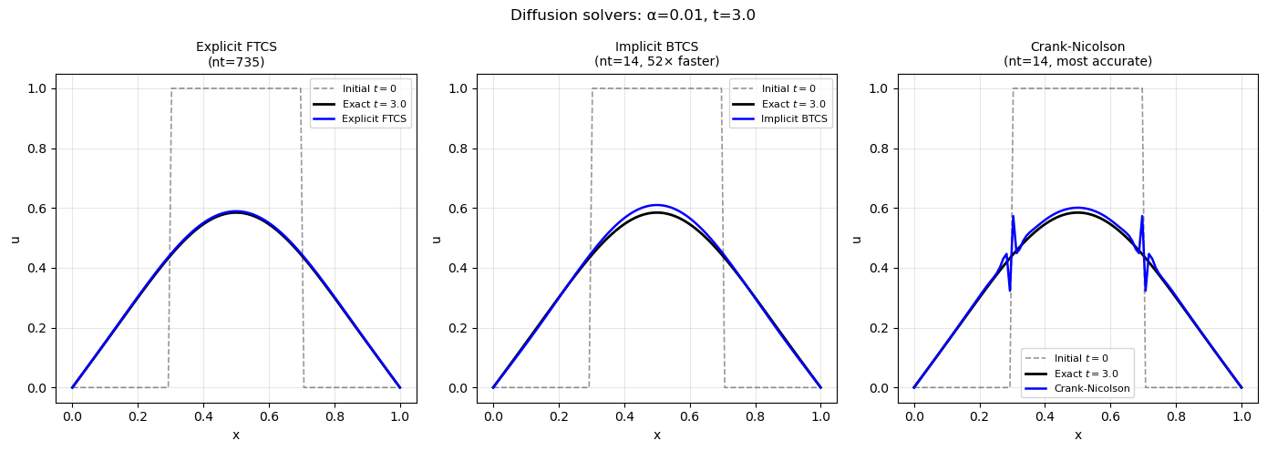
print('=== Scheme comparison ===')
print(f'Explicit FTCS:     dt = {dt_expl:.4e} s,  nt = {nt_expl:6d} steps')
print(f'Implicit BTCS:     dt = {dt_impl:.4e} s,  nt = {nt_impl:6d} steps  ({nt_expl//nt_impl}× fewer!)')
print(f'Crank-Nicolson:    dt = {dt_impl:.4e} s,  nt = {nt_impl:6d} steps')
print()
print('L2 errors vs exact:')
for name, u_num in [('Explicit FTCS', u_expl), ('Implicit BTCS', u_btcs), ('Crank-Nicolson', u_cn)]:
    err = np.sqrt(np.mean((u_num - u_exact)**2))
    print(f'  {name:20s}: {err:.5f}')
print()
print('CN has the same number of time steps as BTCS but better accuracy')
print('because it is second-order in time (BTCS is first-order).')

# ── Plots ─────────────────────────────────────────────────────────────────────
fig, axes = plt.subplots(1, 3, figsize=(14, 5))

for ax, u_num, label in zip(axes,
    [u_expl, u_btcs, u_cn],
    [f'Explicit FTCS\n(nt={nt_expl})',
     f'Implicit BTCS\n(nt={nt_impl}, {nt_expl//nt_impl}× faster)',
     f'Crank-Nicolson\n(nt={nt_impl}, most accurate)']):

    ax.plot(x, u0,      'k--', lw=1.2, alpha=0.4, label='Initial $t=0$')
    ax.plot(x, u_exact, 'k-',  lw=2,              label=f'Exact $t={T_end}$')
    ax.plot(x, u_num,   'b-',  lw=1.8,             label=label.split('\n')[0])
    ax.set_title(label, fontsize=10)
    ax.set_xlabel('x'); ax.set_ylabel('u')
    ax.legend(fontsize=8); ax.grid(True, alpha=0.3)

plt.suptitle(f'Diffusion solvers: α={alpha}, t={T_end}', fontsize=12)
plt.tight_layout()
plt.show()

=== Scheme comparison ===
Explicit FTCS:     dt = 4.0812e-03 s,  nt =    735 steps
Implicit BTCS:     dt = 2.0406e-01 s,  nt =     14 steps  (52× fewer!)
Crank-Nicolson:    dt = 2.0406e-01 s,  nt =     14 steps

L2 errors vs exact:
  Explicit FTCS       : 0.00343
  Implicit BTCS       : 0.01276
  Crank-Nicolson      : 0.02598

CN has the same number of time steps as BTCS but better accuracy
because it is second-order in time (BTCS is first-order).

4. Von Neumann Stability Analysis — Proving $r \leq 1/2$

The method

Assume the error grows as a Fourier mode: $\epsilon^n_i = G^n e^{ik_m i \Delta x}$ where $G$ is the amplification factor. Substitute into the scheme and solve for $G$.

Stability condition: $|G| \leq 1$ for all wavenumbers $k_m$.

For explicit FTCS

Substituting into $u^{n+1}_i = u^n_i + r(u^n_{i+1}-2u^n_i+u^n_{i-1})$:

$G = 1 + r(e^{ik\Delta x} - 2 + e^{-ik\Delta x}) = 1 + r(2\cos(k\Delta x) - 2) = 1 - 4r\sin^2\!\left(\frac{k\Delta x}{2}\right)$

For stability: $|G| \leq 1$, i.e. $-1 \leq 1 - 4r\sin^2(\theta) \leq 1$.

The upper bound gives $r \geq 0$ (always true). The lower bound gives:

$1 - 4r\sin^2(\theta) \geq -1 \implies r \leq \frac{1}{2\sin^2(\theta)} \geq \frac{1}{2}$

Worst case ($\theta = \pi/2$, the shortest resolved wave): $r \leq 1/2$.

For implicit BTCS

$G = \frac{1}{1 + 4r\sin^2(k\Delta x/2)}$

Since the denominator $\geq 1$ always, $|G| \leq 1$ for all $r$ — unconditionally stable.

Summary

In the Navier-Stokes solver (Module 2): Viscous terms are discretised implicitly (BTCS or CN) to avoid the $r \leq 1/2$ constraint — otherwise near-wall cells with tiny $\Delta y$ would force microsecond time steps on a flow that takes seconds to develop.

Next: Module 1.8 — 1D Burgers' Equation: combining advection and diffusion, introducing nonlinearity, and witnessing shock formation.