Higher-Order Schemes
Lesson 3.4 of the CFD for Absolute Beginners course — Higher-Order Schemes.
Lesson 3.4 — Higher-Order Schemes and TVD Limiters
The Dispersion-Diffusion Dilemma
Recall from Lesson 1.6:
- First-order upwind: stable but diffusive (smears sharp features)
- Second-order central: accurate but dispersive (creates oscillations near discontinuities)
The ideal scheme: second-order accuracy in smooth regions, non-oscillatory near shocks. This is what TVD (Total Variation Diminishing) schemes provide.
Total Variation
The total variation of a discrete solution is:
A scheme is TVD if — the solution cannot develop new local extrema.
Godunov's theorem: linear schemes that are both TVD and second-order accurate do not exist. Solution: use nonlinear schemes that adapt their order depending on the local smoothness.
Flux Limiters
A TVD scheme writes the face flux as:
where is the limiter function and is the ratio of consecutive gradients:
| Limiter | Property | |
|---|---|---|
| Minmod | Most diffusive TVD | |
| Van Leer | Smooth, second-order | |
| Superbee | Least diffusive TVD | |
| MC (monotonized central) | Good all-round |
When (smooth region): → second-order accuracy.
When (local extremum): → first-order (non-oscillatory).
QUICK Scheme
QUICK (Quadratic Upstream Interpolation for Convective Kinematics, Leonard 1979) uses a quadratic interpolation:
This is third-order accurate in smooth regions but not TVD — it can create overshoots near shocks.
import numpy as np
import matplotlib.pyplot as plt
# Compare schemes on advection of a step function (discontinuity + smooth region)
def advect_scheme(u0, c, dx, dt, nt, scheme='upwind'):
u = u0.copy()
nu = c * dt / dx
for _ in range(nt):
u_old = u.copy()
if scheme == 'upwind':
u[1:] = u_old[1:] - nu*(u_old[1:] - u_old[:-1])
u[0] = u_old[0] - nu*(u_old[0] - u_old[-1])
elif scheme == 'lax_wendroff':
u[1:-1] = (u_old[1:-1]
- nu/2*(u_old[2:] - u_old[:-2])
+ nu**2/2*(u_old[2:] - 2*u_old[1:-1] + u_old[:-2]))
u[0] = u_old[0]
u[-1] = u_old[-1]
elif scheme in ('minmod', 'van_leer', 'superbee', 'mc'):
# TVD with flux limiter
def limiter(r, name):
if name == 'minmod':
return np.maximum(0, np.minimum(1, r))
elif name == 'van_leer':
return (r + np.abs(r)) / (1 + np.abs(r) + 1e-12)
elif name == 'superbee':
return np.maximum(0, np.maximum(np.minimum(2*r, 1), np.minimum(r, 2)))
elif name == 'mc':
return np.maximum(0, np.minimum(np.minimum(2*r, 0.5*(1+r)), 2))
u_new = np.zeros_like(u_old)
# Extended array for periodic BCs
ue = np.concatenate([u_old[-2:], u_old, u_old[:2]])
for i in range(len(u_old)):
i_e = i + 2 # offset in extended array
# r at right face
denom = ue[i_e+1] - ue[i_e] + 1e-12
r_right = (ue[i_e] - ue[i_e-1]) / denom
phi_right = limiter(r_right, scheme)[0] if hasattr(r_right, '__len__') else limiter(np.array([r_right]), scheme)[0]
F_right = c*(ue[i_e] + 0.5*phi_right*(1-nu)*(ue[i_e+1]-ue[i_e]))
denom_l = ue[i_e] - ue[i_e-1] + 1e-12
r_left = (ue[i_e-1] - ue[i_e-2]) / denom_l
phi_left = limiter(r_left, scheme)[0] if hasattr(r_left, '__len__') else limiter(np.array([r_left]), scheme)[0]
F_left = c*(ue[i_e-1] + 0.5*phi_left*(1-nu)*(ue[i_e]-ue[i_e-1]))
u_new[i] = u_old[i] - nu*(F_right - F_left)/c
u = u_new
return u
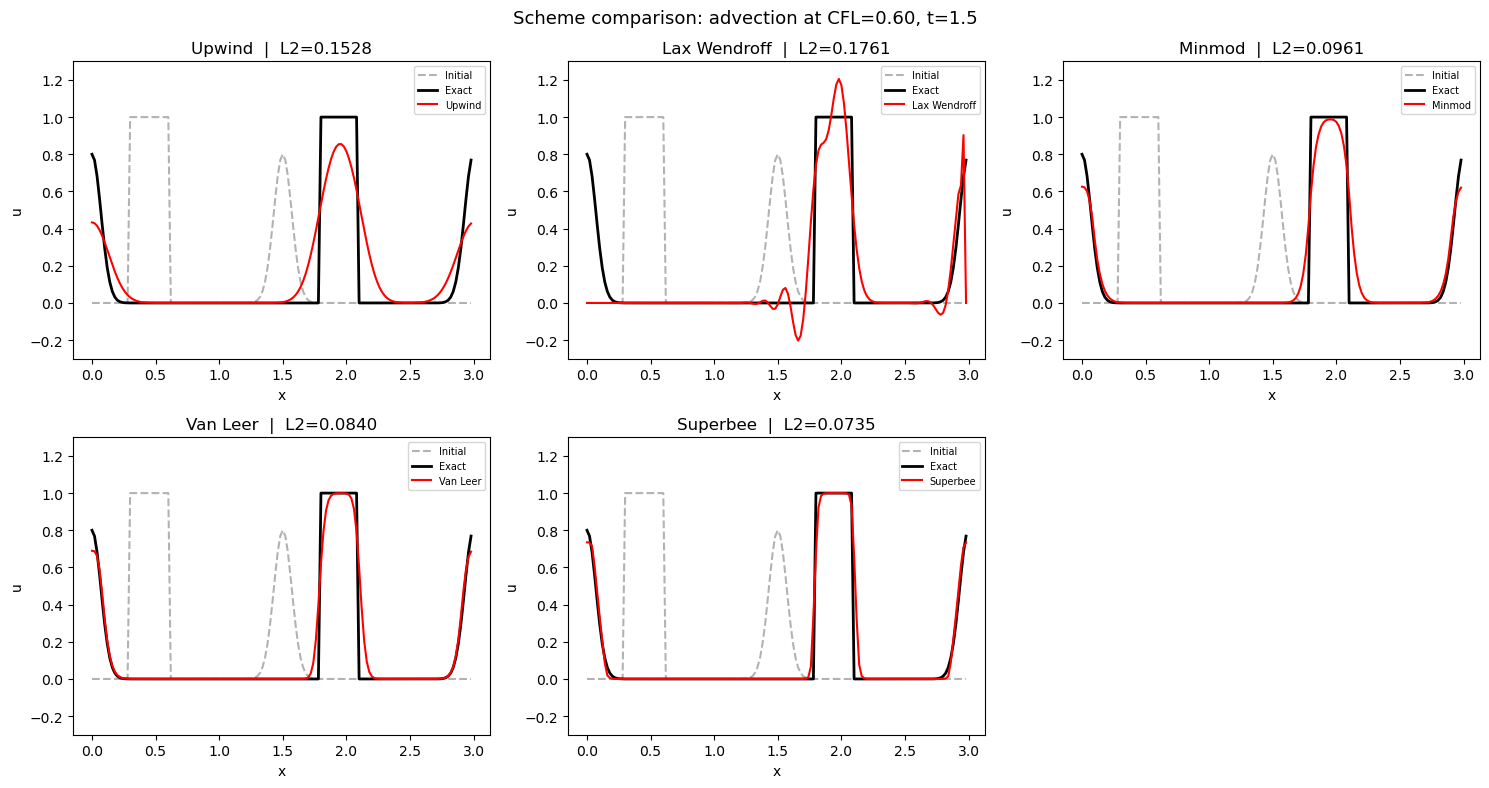
# Setup: mixed initial condition (step + smooth Gaussian)
N = 150
L = 3.0
dx = L / N
x = np.linspace(0, L, N, endpoint=False)
c = 1.0
dt = 0.6 * dx / c
T = 1.5
nt = int(T / dt)
# Step + Gaussian
u0 = np.zeros(N)
u0[(x >= 0.3) & (x <= 0.6)] = 1.0 # step
u0 += 0.8 * np.exp(-((x - 1.5)**2) / 0.01) # Gaussian
x_exact = (x - c*T) % L
u_exact = np.zeros(N)
u_exact[(x_exact >= 0.3) & (x_exact <= 0.6)] = 1.0
u_exact += 0.8 * np.exp(-((x_exact - 1.5)**2) / 0.01)
schemes = ['upwind', 'lax_wendroff', 'minmod', 'van_leer', 'superbee']
results = {s: advect_scheme(u0, c, dx, dt, nt, s) for s in schemes}
fig, axes = plt.subplots(2, 3, figsize=(15, 8))
axes_flat = axes.ravel()
for ax, scheme in zip(axes_flat, schemes):
ax.plot(x, u0, 'k--', alpha=0.3, linewidth=1.5, label='Initial')
ax.plot(x, u_exact, 'k-', linewidth=2, label='Exact')
ax.plot(x, results[scheme], 'r-', linewidth=1.5, label=scheme.replace('_', ' ').title())
l2 = np.sqrt(np.mean((results[scheme] - u_exact)**2))
ax.set_title(f'{scheme.replace("_"," ").title()} | L2={l2:.4f}')
ax.set_xlabel('x'); ax.set_ylabel('u')
ax.legend(fontsize=7); ax.set_ylim(-0.3, 1.3)
axes_flat[-1].axis('off')
plt.suptitle(f'Scheme comparison: advection at CFL={c*dt/dx:.2f}, t={T}', fontsize=13)
plt.tight_layout()
plt.show()
Sweby Diagram
Plot vs for all limiters. A scheme is TVD if its limiter lies within the Sweby region:
r = np.linspace(-0.5, 3.5, 500)

limiters = {
    'Minmod': np.maximum(0, np.minimum(1, r)),
    'Van Leer': (r + np.abs(r)) / (1 + np.abs(r) + 1e-12),
    'Superbee': np.maximum(0, np.maximum(np.minimum(2*r, 1), np.minimum(r, 2))),
    'MC': np.maximum(0, np.minimum(np.minimum(2*r, 0.5*(1+r)), 2)),
    'QUICK': 0.75 + 0.25*r,  # QUICK limiter (not TVD — can be outside region)
}

# Sweby region bounds
upper = np.maximum(0, np.maximum(np.minimum(2*r, 1), np.minimum(r, 2)))
lower = np.zeros_like(r)

fig, ax = plt.subplots(figsize=(8, 7))
ax.fill_between(r, lower, upper, alpha=0.15, color='green', label='Sweby TVD region')

colors = ['blue', 'red', 'purple', 'orange', 'gray']
for (name, phi), color in zip(limiters.items(), colors):
    ax.plot(r, phi, color=color, linewidth=2, label=name)

ax.axhline(0, color='k', linewidth=0.5)
ax.axvline(0, color='k', linewidth=0.5)
ax.axvline(1, color='k', linewidth=0.5, linestyle=':')
ax.set_xlabel('$r$ (gradient ratio)', fontsize=12)
ax.set_ylabel('$\\phi(r)$ (limiter value)', fontsize=12)
ax.set_title('Sweby diagram: TVD limiters', fontsize=13)
ax.legend(fontsize=10)
ax.set_xlim(-0.5, 3.5); ax.set_ylim(-0.2, 2.5)
ax.grid(True, alpha=0.3)
ax.text(1.05, 0.85, 'Second-order\nlocus', fontsize=9, color='green')
plt.tight_layout()
plt.show()

print("Limiters inside Sweby region → TVD (no new oscillations).")
print("QUICK extends outside → not TVD (overshoots near discontinuities).")
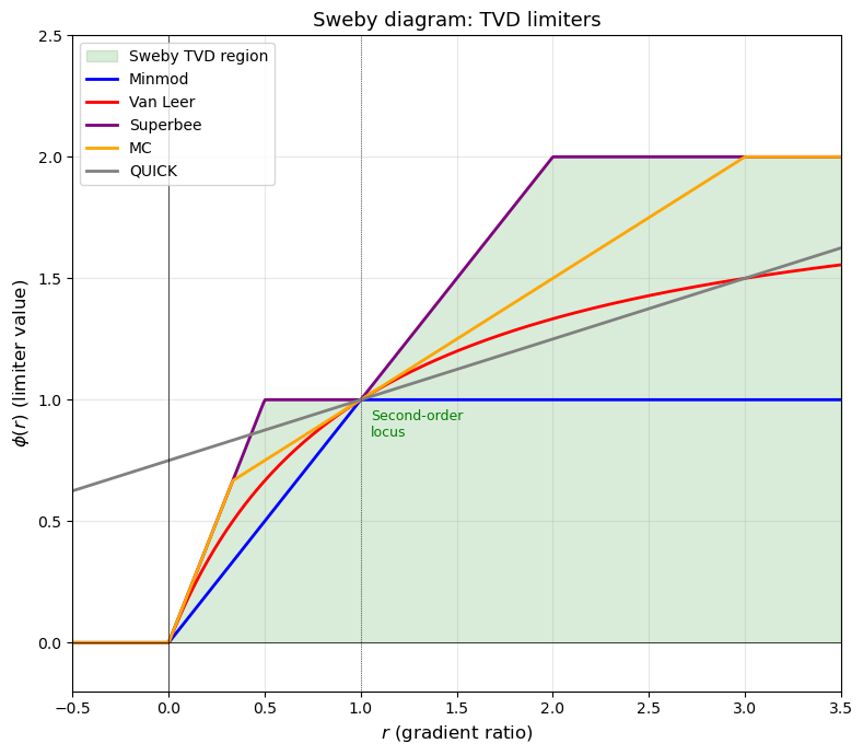
Limiters inside Sweby region → TVD (no new oscillations).
QUICK extends outside → not TVD (overshoots near discontinuities).
Key Takeaways
- First-order upwind: diffusive. Second-order central/Lax-Wendroff: oscillatory near discontinuities.
- TVD schemes use flux limiters to be second-order in smooth regions, first-order near shocks.
- Godunov's theorem: no linear scheme is both second-order and TVD — limiters are nonlinear.
- Limiter choice: Minmod (most diffusive), Van Leer (smooth), Superbee (sharpest — can be over-compressive).
- In OpenFOAM:
limitedLinear(Van Leer-like),limitedLinearVfor vectors.
Next: Lesson 3.5 — Multigrid Methods: V-cycle, convergence acceleration.