Module 1.4 — The Continuity Equation

Why dedicate a full module to one equation? The continuity equation is two lines long and looks trivial. But $\nabla\cdot\mathbf{u}=0$ is the constraint that makes incompressible CFD hard. Every instability in the pressure solver, every checkerboard pressure mode, every diverging SIMPLE iteration — all of it traces back to this one equation not being satisfied properly.

Understanding it deeply now means every pressure-solver difficulty you encounter later will have a clear diagnosis.

Roadmap:

1. Derivation — where the equation comes from, physically
2. Incompressible form and what it means geometrically
3. The streamfunction — a tool that satisfies continuity automatically
4. Divergence-free vs. non-divergence-free fields — what they look like
5. Why incompressible pressure is not thermodynamic
6. Python: checking, enforcing, and visualising divergence

import numpy as np
import matplotlib.pyplot as plt

1. Derivation — The Pipe Cross-Section Argument

The highway analogy

Imagine a single-lane highway. At a given moment, the density of cars (cars per km) and their speed determine the car flux (cars per hour passing a point). If cars flow into a stretch of highway faster than they leave, density builds up — a traffic jam forms. If they leave faster, the stretch empties.

The continuity equation says exactly this for a fluid, with density replacing car density:

$\underbrace{\frac{\partial \rho}{\partial t}}_{\substack{\text{density builds up}\\\text{or depletes}}} + \underbrace{\frac{\partial(\rho u)}{\partial x}}_{\substack{\text{gradient of mass flux}\\\text{(more leaving than entering)}}} = 0$

Step-by-step 3D derivation

Take a small rectangular control volume $\Delta x \times \Delta y \times \Delta z$.

x-direction: mass flux in minus mass flux out: $(\rho u)|_x \, \Delta y \Delta z \, \Delta t - (\rho u)|_{x+\Delta x} \, \Delta y \Delta z \, \Delta t \approx -\frac{\partial(\rho u)}{\partial x} \Delta x \Delta y \Delta z \Delta t$

The same applies in $y$ and $z$. The total change in mass inside the CV must equal the net flux in:

$\frac{\partial \rho}{\partial t} \Delta x \Delta y \Delta z = -\left(\frac{\partial(\rho u)}{\partial x} + \frac{\partial(\rho v)}{\partial y} + \frac{\partial(\rho w)}{\partial z}\right) \Delta x \Delta y \Delta z$

Divide by $\Delta x \Delta y \Delta z$:

$\boxed{\frac{\partial \rho}{\partial t} + \nabla \cdot (\rho \mathbf{u}) = 0}$

No approximations. This is exact.

2. The Incompressible Form — What It Means Geometrically

When is $\rho =$ const valid?

Expand $\nabla\cdot(\rho\mathbf{u}) = \rho\nabla\cdot\mathbf{u} + \mathbf{u}\cdot\nabla\rho$. If $\rho$ changes negligibly:

$\nabla\cdot\mathbf{u} = 0$

This is valid when:

• Liquids (water, oil): density varies less than 0.01% with typical pressure changes
• Slow gases ($M < 0.3$): density changes are smaller than 5% of the reference density
• Non-buoyant flows: temperature variations don't cause significant density changes

Rule of thumb: if the flow speed is less than 30% of the speed of sound, treat it as incompressible.

Geometric interpretation

Consider a small fluid parcel (a tiny cube of fluid). As it moves:

• If $\nabla\cdot\mathbf{u} > 0$: the parcel is expanding (fluid diverges from it)
• If $\nabla\cdot\mathbf{u} < 0$: the parcel is compressing (fluid converges toward it)
• If $\nabla\cdot\mathbf{u} = 0$: the parcel's volume is preserved as it moves

Incompressible flow = every fluid parcel conserves its volume as it moves through the domain. Fluid can be stretched and sheared (changing shape), but not compressed or expanded.

In 2D — the four-neighbour constraint

$\frac{\partial u}{\partial x} + \frac{\partial v}{\partial y} = 0$

If flow accelerates in $x$ ($\partial u/\partial x > 0$, e.g. a converging channel), it must decelerate in $y$ ($\partial v/\partial y < 0$) to compensate. The two velocity components are not independent — they are tied together by this constraint. This is why solving incompressible N-S requires a separate step to enforce continuity (the pressure Poisson equation).

3. The Streamfunction — Automatic Continuity Satisfaction

The clever trick

For 2D incompressible flow, define a scalar function $\psi(x, y)$ such that:

$u = \frac{\partial \psi}{\partial y}, \qquad v = -\frac{\partial \psi}{\partial x}$

Substituting into the continuity equation:

$\frac{\partial u}{\partial x} + \frac{\partial v}{\partial y} = \frac{\partial^2\psi}{\partial x \partial y} - \frac{\partial^2\psi}{\partial y \partial x} = 0 \checkmark$

Any smooth $\psi$ automatically satisfies continuity. You can choose $\psi$ freely and always get a valid incompressible velocity field from it.

Why streamlines are contours of $\psi$

Along a streamline, the velocity is tangent to the curve. The condition for a curve $f(x,y) = \text{const}$ to be a streamline is:

$u \frac{\partial f}{\partial y} - v \frac{\partial f}{\partial x} = 0$

Substituting $u = \partial\psi/\partial y$ and $v = -\partial\psi/\partial x$ shows that $f = \psi$ satisfies this exactly. Contours of $\psi$ are streamlines.

Practical consequence: when you visualise CFD results with ax.contour(X, Y, psi, ...), you are plotting the exact streamlines of the flow. The spacing between streamlines tells you the speed — closely spaced streamlines = high velocity (by continuity, same mass must pass through a narrow gap).

Physical meaning of $\psi$

The difference in $\psi$ between two streamlines equals the volumetric flow rate (per unit depth) between them:

$Q_{1\to 2} = \psi_2 - \psi_1 \quad \text{[m²/s per unit depth]}$

This is useful for computing flow rates directly from the visualisation.

# ── The streamfunction in action ─────────────────────────────────────────────
# Start with an arbitrary streamfunction, derive u and v,
# then verify that div(u) = 0 exactly.

# ── Grid ────────────────────────────────────────────────────────────────────
N  = 80
x  = np.linspace(0, 2, N);   dx = x[1]-x[0]
y  = np.linspace(0, 1, N);   dy = y[1]-y[0]
X, Y = np.meshgrid(x, y)

# ── Choose a streamfunction (arbitrary smooth function) ─────────────────────
# ψ = sin(πx)·sin(πy): corresponds to a single vortex in a box
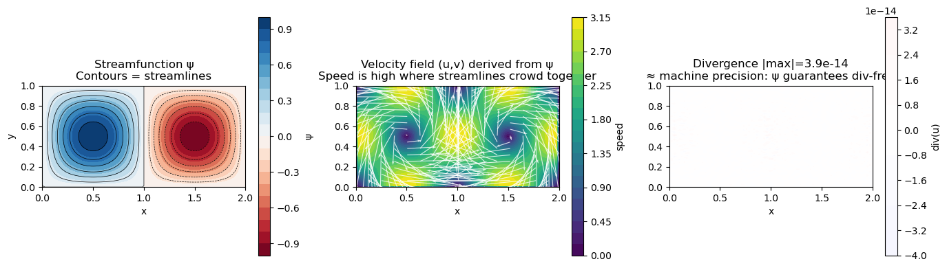
psi = np.sin(np.pi * X) * np.sin(np.pi * Y)

# ── Derive velocity from streamfunction ─────────────────────────────────────
# u = ∂ψ/∂y  (central differences)
# v = -∂ψ/∂x
U = np.zeros_like(psi)
V = np.zeros_like(psi)
U[1:-1, :] = (psi[2:, :] - psi[:-2, :]) / (2*dy)     # ∂ψ/∂y
V[:, 1:-1] = -(psi[:, 2:] - psi[:, :-2]) / (2*dx)    # -∂ψ/∂x

# ── Check divergence ────────────────────────────────────────────────────────
div = np.zeros_like(U)
div[1:-1, 1:-1] = ((U[1:-1, 2:] - U[1:-1, :-2]) / (2*dx) +
                   (V[2:, 1:-1] - V[:-2, 1:-1]) / (2*dy))

print('=== Streamfunction verification ===')
print(f'ψ = sin(πx)·sin(πy)')
print(f'u = ∂ψ/∂y = π·sin(πx)·cos(πy)')
print(f'v = -∂ψ/∂x = -π·cos(πx)·sin(πy)')
print()
print(f'Max |div(u)|: {np.max(np.abs(div[1:-1,1:-1])):.2e}')
print(f'  → ~machine precision: any ψ gives a divergence-free field automatically')
print()
print('Flow rate between ψ=0 (walls) and ψ=max (centre streamline):')
print(f'  Q = ψ_max - ψ_min = {psi.max():.4f} - {psi.min():.4f} = {psi.max()-psi.min():.4f} m²/s per unit depth')

# ── Visualise ────────────────────────────────────────────────────────────────
fig, axes = plt.subplots(1, 3, figsize=(14, 4))

# Streamfunction
cf = axes[0].contourf(X, Y, psi, levels=20, cmap='RdBu')
plt.colorbar(cf, ax=axes[0], label='ψ')
axes[0].contour(X, Y, psi, levels=15, colors='k', linewidths=0.5)
axes[0].set_title('Streamfunction ψ\nContours = streamlines'); axes[0].set_aspect('equal')
axes[0].set_xlabel('x'); axes[0].set_ylabel('y')

# Velocity field
speed = np.sqrt(U**2 + V**2)
skip = 5
cf2 = axes[1].contourf(X, Y, speed, levels=20, cmap='viridis')
plt.colorbar(cf2, ax=axes[1], label='speed')
axes[1].quiver(X[::skip,::skip], Y[::skip,::skip],
               U[::skip,::skip], V[::skip,::skip], color='white', alpha=0.8, scale=8)
axes[1].set_title('Velocity field (u,v) derived from ψ\nSpeed is high where streamlines crowd together')
axes[1].set_aspect('equal'); axes[1].set_xlabel('x')

# Divergence — should be ~zero
cf3 = axes[2].contourf(X, Y, div, levels=20, cmap='bwr', vmin=-1e-12, vmax=1e-12)
plt.colorbar(cf3, ax=axes[2], label='div(u)')
axes[2].set_title(f'Divergence |max|={np.max(np.abs(div[1:-1,1:-1])):.1e}\n≈ machine precision: ψ guarantees div-free')
axes[2].set_aspect('equal'); axes[2].set_xlabel('x')

plt.tight_layout()
plt.show()

=== Streamfunction verification ===
ψ = sin(πx)·sin(πy)
u = ∂ψ/∂y = π·sin(πx)·cos(πy)
v = -∂ψ/∂x = -π·cos(πx)·sin(πy)

Max |div(u)|: 3.86e-14
  → ~machine precision: any ψ gives a divergence-free field automatically

Flow rate between ψ=0 (walls) and ψ=max (centre streamline):
  Q = ψ_max - ψ_min = 0.9996 - -0.9996 = 1.9992 m²/s per unit depth

4. Why Incompressible Pressure Is Not Thermodynamic

The surprise

In compressible flow, pressure is a thermodynamic quantity: it comes from an equation of state ($p = \rho R T$ for an ideal gas). You compute $p$ from $\rho$ and $T$.

In incompressible flow, there is no equation of state for pressure. Density is constant and temperature (if energy is decoupled) is irrelevant to the momentum balance. So where does $p$ come from?

Pressure as a constraint enforcer

Think of it this way: the momentum equation will give you a velocity field, but that velocity field will generally not satisfy $\nabla\cdot\mathbf{u}=0$. Pressure adjusts — instantaneously, infinitely fast — to correct the velocity so that it becomes divergence-free.

Mathematically, $p$ is a Lagrange multiplier that enforces the incompressibility constraint.

This is derived by taking the divergence of the momentum equation and using $\nabla\cdot\mathbf{u}=0$:

$\nabla^2 p = -\rho \nabla\cdot[(\mathbf{u}\cdot\nabla)\mathbf{u}]$

This is the pressure Poisson equation (Module 2.4). Given the velocity, solve this for $p$; then use $p$ to correct the velocity so it becomes divergence-free.

Consequences

1. Pressure propagates at infinite speed in incompressible flow. A perturbation at one point is felt everywhere instantly. (In compressible flow it travels at the speed of sound.)

2. Pressure is determined only up to an additive constant. You must fix it at one point (or remove the mean) to get a unique solution.

3. Absolute pressure values don't matter — only pressure gradients drive the flow. You can shift $p$ by any constant without changing $\mathbf{u}$.

Summary

Next: Module 1.5 — Finite Difference Method: Taylor series, truncation error, and the stencils that discretise every derivative in this curriculum.

Exercise

Predict first, then verify.

1. Is the velocity field $u = \cos(x)\sin(y)$, $v = \sin(x)\cos(y)$ incompressible? Compute $\partial u/\partial x + \partial v/\partial y$ analytically first, then verify numerically.

2. Construct a streamfunction $\psi = x^2 y - y^3/3$ (a classic corner flow). Derive $u$ and $v$, verify incompressibility, and plot the streamlines. What kind of flow does this represent?

3. For the streamfunction in part (2), compute the volumetric flow rate between the streamlines $\psi = 0$ and $\psi = 1$ at $x = 1$.